Stock Analysis
Link to Project Log: Stock Analysis Log
Link to GitHub [1]
Project Overview
The financial market is an extremely complicated place. While there are many metrics used to measure the health of markets, market values such as the S&P 500, Russell 2000, and the Dow Jones Industrial average are the ones that we will focus on. We will build models of the market so that users can input how they think the interest rate, unemployment rate, price of gold, and other factors will change, and our models will predict how the market will react to those changes. The user will enter their predictions into a user interface, and the product will output visual aid as well as estimated prices and behavior. Our product will help users make more informed investment decisions.
Group Members
- Brandt Lawson
- Keith Kamons
- Jessica
- Chang Xue (TA)
Objectives
Produce a user interface which, given a user specified value for some factors, can predict what impact this change will have on future index values. The accuracy and precision of the model can be determine through back testing and measure the success of the project. We will demonstrate our project by allowing users to predict changes in many factors and to see how our model does at predicting the markets reaction.
Challenges
- Learning how to use MySQL.
- The web security behind sharing data online and how to accomplish this in a safe and secure way.
- Learning how to use Python's data analysis toolboxes.
- Nobody in the group has taken a course or studied how many of the analysis tools and underlying math and computer science works, so it will be incredibly challenging to figure it all out along the way.
- Integrating this software across different platforms and allowing everyone in the group to have access to this data.
- Data collection and storage in an efficient and complete way
- Collecting data in an autonomous and dynamic way will be a challenge due to the ways that resources such as Google Finance, Yahoo Finance and Quandl change their policies on data collection.
- Manual data collection and cleaning while the code for autonomous collection and analysis is setup.
Gantt Chart
Budget
Our goal is to exclusively use open source data and software, which makes our budget $0.00.
Data
Data Collection
First we used a Bloomberg terminal to extract historical price data on the S&P 500 and several features and commodities. See the guide on how to do so here: Bloomberg Data Extraction
Data Storage
Once the data was collected, we exported the data to an excel file for processing [2].
App Prototype
Design & Solutions
The Data Management
One of the biggest challenges we faced was in data collection and management. Originally we intended on using an API to dynamically fetch data and store it in a MySQL database we configured on an Amazon EC2 Micro Instance. We attempted to use Quandl, GoogleFinance, and YahooFinance's APIs but they were decommissioned so we were unable to utilize them.[3][4] [5] To resolve this issue, we wrote a web scraper in Python that read data from several Google Finance web pages, but ultimately our requests to the web pages were blocked by Google. This forced us to reconsider how we should collect and store data. Our workaround for this issue was to keep our data set static and to collect our data from the Bloomberg terminal.
The results generated for the output relied on historical pricing of market indicators and indices. We collected pricing data on several commodities, indices, and indicators through a Bloomberg terminal. This posed as a challenge for us because the Bloomberg terminal has a large amount of data for each price we examined. We had to research the syntax of tickers and how to understand the long-term contracts involved so we could pull the pricing data. We then exported and stored the data in an excel workbook.
After collection, the data was then processed using Python's sklearn preprocessor, pandas and numpy toolboxes [6]. The data from the year 1980 through 2018 was collected, but data did not exist for every day in the range, so there were holes in the data set or entries that were left as not available (#N/A). These are the points we had to fix in the data set. By storing the data in a pandas data frame we were able to iterate over the data set and process all of the improperly formatted points by replacing them with a standard (#N/A) message. Sklearn and ARIMA toolboxes were able to handle this standard error message. Additionally, we used interest and unemployment rates as features. This type of data is reported once every quarter, so there were many entries left as (#N/A). We handled this by assuming that the unemployment and interest rates do not change between the time are reported. Realistically these rates change dynamically in real time, but they generally hover around the reported rates.
The Statistical Analysis
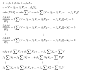
As part of our objective, we want to identify how some change in a variable, say GDP, effects the overall price of the S&P 500. In order to accomplish this we needed to determine what relationships exist between features and the price of the S&P 500, as well as the relationships between features themselves. Linear regression quantifies these relationships for us. As part of our data exploration, we constructed a correlation matrix and plotted a line of best fit using the L2 loss function. Using this visualization, we can saw that certain variables are strongly correlated to S&P 500 price both positively and negatively, and some have a weak correlation. We also observe that certain features are highly correlated to each other. We avoided using highly correlated features as this can damage the model.
In order to test how well the model performed, we devised a method of testing using past data. The traditional method consists of a training-test split, where the model is trained on the first 70% of the data and then its predictions compared to the target variable from the latter 30%. We took this idea, and modified it in order to attain a more generalized model, and to account for the time series nature of our data. Our splits consist of taking the first 20 percent of data to train-test, then rolling forward the data we select to train-test. We also set a max training data length, so as to avoid training on older data.
Running OLS regression through this cross validation, we got results that were not great. This is likely due to the fact that we are using only a few features while in reality there are millions of features and interactions behind the S&P 500. After trying a few other models for comparison, we found the ARIMA (Autoregressive, integrated, moving average) model gave us much best results [7]. ARIMA uses historical target variable values as its features. We still wanted to be able to analyze the component wise effect of the features on the S&P 500, so we came up with a way to utilize both models to give us this functionality. The change in predicted price using OLS regression before and after changing a feature value was reasonable; the only problem was the overall bias of the value was undervalued. Since ARIMA gives us a reasonable price, we can simple run ARIMA, and then add the delta predicted via OLS corresponding to the users change in the feature. Both back testing and visualizing this method confirms it works!
Modeling a system as efficient as the stock market is tricky. If predicting the future prices of securities with certainty was as easy as a few regressions, we would not be in school right now. As soon as any simple relationship exists, someone would have already figured it out and arbitraged away any mis-pricing. The pricing we are then left with is essentially random for the short run. This is why our model cannot perfectly predict the market, but can make reasonable guesses or medium time horizons.
The Graphical User Interface
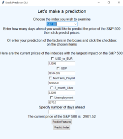
We created a GUI using Python's Tkinter toolbox. We modeled our GUI after the Programming GUIs and windows with Tkinter and Python [8] embedded with the functions as mentioned above. The GUI consisted of a single frame which was updated based on user inputted data.
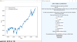
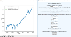
The main page displayed the current prices of the features and index being examined. The page was generated iteratively based off of the excel file that the data was stored in. This allows for the information to be changed dynamically in the future. Users have two options. First, the user could input a number of days, then let the model predict the price of the S&P 500 along with the features and a visualization in the specified number of days. Secondly, the user can choose which features they think will change and enter in their prediction. The model will then output the forecasted price of the S&P 500 based on the users changes. This data is plotted with predicted price of the S&P 500 in the specified number of days to see how the user's prediction aligns with the models prediction based on no change.
Bloomberg Data Extraction
Learn how to extract data from a Bloomberg terminal here: Bloomberg Data Extraction.
Results
Comparison to Objectives
Our project met our objectives and goals. We successfully created a user interface that allows users to predict feature and index prices as well as calculate the impact that changes in feature price will have on future values of an index. The interface outputs a visualization of the index's behavior as well as a specific estimate for the price. Additionally, we included a feature that allows the user to specify the number of days ahead they wish to predict the values of the index.
The features we used were the US Dollar to Euro currency exchange rate, gross domestic product, nonfarm payroll, 3 month LIBOR, and the unemployment rate. The interface allows the user to select a combination of features and makes a prediction based on the number of days ahead, or based off the the user inputted change in feature price and number of days ahead. The visualization depicts the prediction given the users input and displays the past values of the index in blue, the predicted price with no change in feature prices in orange, and the prediction with change in feature price in green. The interface itself also updates the feature prices in the text boxes if the prediction is made with no change in feature price.
Source Code: GitHub
Critical Decisions
We originally set out to have a dynamic stream of data that would change our results on a day by day basis. This would have required use of an API, or a subscription to a financial service provider like Bloomberg. We decided against using an API because the Google Finance and Yahoo Finance APIs were not well maintained and could not be implemented. We wrote our own web scraper, which collected data from both Google Finance and Yahoo Finance web pages. Our IP address was blocked from making so many requests which made this option infeasible. A subscription to a financial service like Bloomberg comes at a cost of $24,000 per year, which is not within the budget of this class.[9] For these reasons we ultimately decided against having a dynamic stream of data and used a static data set.
Additionally, we wanted to let the user find correlations between and make predictions off of any of the 15 features that we collected data for. This means that there would be 32768 different combinations of features the user could choose from. The modeling that we did was computationally intense and therefore the time needed to run the model increased significantly with the number of features used to predict the price of the index. For this reason, we computed the coefficients used to calculated predictions based off of the users combination of features and stored them in a file to save time when the program was in use. We settled on five features because the number of combinations increases exponentially. The five that we chose were based off of their diversity and how well they correlated to the index we examined.
Next Steps
To expand the usability of our project, we would implement more market indices as well as implement more features. When we trained the model using more features, the program crashed due to the computation time and complexity of the statistical analysis. To implement more features, we would need a computer that can handle significantly more data or we would need to refine the algorithms to make them more efficient. We could also use some type of trick to reduce the number of features we analyze, such as principal component analysis (PCA).
We would also use a dynamic stream of data to allow for updates in real time with current market actions. In order to achieve this, we would have to pay for an API key, or subscribe to a financial service, which has the costs as mentioned above.
After using machine learning, we could implement deep learning for increased accuracy and to allow for a much higher number of interactions between features. For this to work, we would need to have significantly more data.
Poster
References
Not Quoted
CSE330 Linux, SQL and AWS info
Python Machine Learning (Sebastian Raschka) 2nd Edition ISBN-10: 1787125939
SciKit Learn SVM Documentation


