Use the sineButterworthFilter function to apply a sine-Butterworth filtering operation to a previously saved X–Y data object (a collection of ordered pairs) to produce a new X–Y data object. This filtering operation can be used, for example, to remove high-frequency noise.
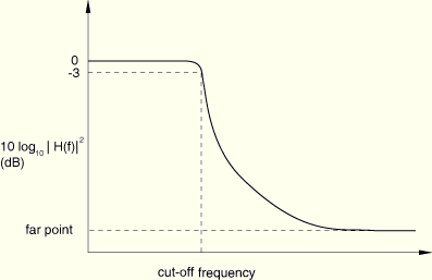
ABAQUS/CAE uses a sine-Butterworth filter whose transfer function ![]() has the following form:
has the following form:
For the filter to be applied to a curve, the curve must have data points at regularly spaced intervals in time. Therefore, a curve to be filtered is resampled at a given frequency (the sampling frequency). The default sampling frequency will be inadequate for curves containing data with a frequency content that is much higher than the cut-off frequency. Using a very high sampling frequency will create a curve with a very large number of data points.
The sineButterworthFilter requires two arguments: the name of the X–Y data object and the cut-off frequency, which is the frequency above which the filter attenuates at least half of the input signal. A description of the optional arguments follows:
The order of the filter you want to use (filterOrder). This argument must be a positive, even integer value; the default value is 6.
A symbolic constant that specifies the interpolation scheme (interpolation). Valid values for this argument are QUADRATIC, specifying a Lagrange second-order interpolation scheme; CUBIC_SPLINE, specifying a cubic spline interpolation scheme; and LINEAR, specifying a linear interpolation scheme. The default value is QUADRATIC.
The slope of the raw data curve leading up to the first data point (startslope). This argument's default value is 0.0 (for a level slope), and it is used only when interpolation=CUBIC_SPLINE.
The slope of the raw data curve continuing past the final data point (endslope). This argument's default value is 0.0 (for a level slope), and it is used only when interpolation=CUBIC_SPLINE.
Your X–Y data object must have a constant time step for it to be filtered. If the time step is not constant, ABAQUS/CAE computes additional points at constant intervals by interpolation. The constant time step is computed from the sampling frequency according to the following relationship:
![]()
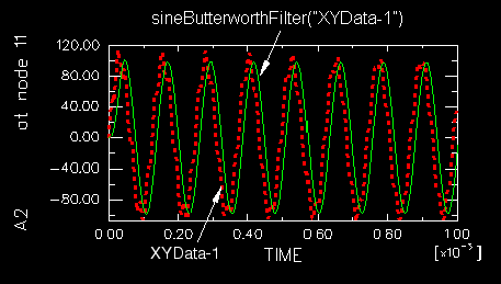
Figure 29–22 illustrates the type of X–Y plot that can be produced using the sineButterworthFilter operation.
To apply sine-Butterworth filtering to an X–Y data object:
Locate the Operate on XY Data dialog box.
From the main menu bar, select Tools![]() XY Data
XY Data![]() Create. Click Operate on XY data in the dialog box that appears; then click Continue. The Operate on XY Data dialog box appears.
Create. Click Operate on XY data in the dialog box that appears; then click Continue. The Operate on XY Data dialog box appears.
From the Operators listed, click sineButterworthFilter(X,F).
The sineButterworthFilter function appears in the expression window.
From the XY Data choices, click the name of the X–Y data object on which to operate and click Add to Expression. You can choose from all X–Y data objects previously saved within this session (listed alphabetically in the XY Data field).
The X–Y data object name appears within the sineButterworthFilter function parentheses in the expression window.
Position the cursor in the expression window before the second comma, and type in a value for the cut-off frequency.
To continue to build your expression, position the cursor in the expression window and type in or select the functions, operators, and X–Y data you want to include.
To evaluate and display your expression, click Plot Expression.
To save your new X–Y data object, click Save As and then provide a name in the dialog box that appears.
Saving your data object makes it available for future operations within this session and for inclusion in X–Y plots containing multiple data objects.
When you are finished, click Cancel to close the dialog box.