26.2.1 Dashpots

Products: ABAQUS/Standard ABAQUS/Explicit ABAQUS/CAE

References

Overview

Dashpot elements:

can couple a force with a relative velocity;
in ABAQUS/Standard can couple a moment with a relative angular velocity;
can be linear or nonlinear;
if linear, can be dependent on frequency in direct-solution steady-state dynamic analysis;
can be dependent on temperature and field variables; and
can be used in any stress analysis procedure.

The terms “force” and “velocity” are used throughout the description of dashpot elements. When the dashpot is associated with displacement degrees of freedom, these variables are the force and relative velocity in the dashpot. If the dashpots are associated with rotational degrees of freedom, they are torsional dashpots; these variables will then be the moment transmitted by the dashpot and the relative angular velocity across the dashpot.

In dynamic analysis the velocities are obtained as part of the integration operator; in quasi-static analysis in ABAQUS/Standard the velocities are obtained by dividing the displacement increments by the time increment.

Typical applications

Dashpots are used to model relative velocity-dependent force or torsional resistance. They can also provide viscous energy dissipation mechanisms.

Dashpots are often useful in unstable, nonlinear, static analyses where the modified Riks algorithm is not appropriate (see “Unstable collapse and postbuckling analysis,” Section 6.2.4, for a discussion of the modified Riks algorithm) and where the automatic time stepping algorithm is used because sudden shifts in configuration can be controlled by the forces that arise in the dashpots. In such cases the magnitude of the damping must be chosen in conjunction with the time period so that enough damping is available to control such difficulties but the damping forces are negligible when a stable static response is obtained. See also the contact damping available with contact elements in ABAQUS/Standard (see “Contact damping,” Section 30.1.3).

Choosing an appropriate element

DASHPOT1 and DASHPOT2 elements are available only in ABAQUS/Standard. DASHPOT1 is between a specified degree of freedom and ground. DASHPOT2 is between two specified degrees of freedom.

The DASHPOTA element is available in both ABAQUS/Standard and ABAQUS/Explicit. DASHPOTA is between two nodes with its line of action being the line joining the two nodes.

The dashpot behavior can be linear or nonlinear in any of these elements.

Input File Usage:

Use the following option to specify a dashpot element between a specified degree of freedom and ground:

*ELEMENT, TYPE=DASHPOT1

Use the following option to specify a dashpot element between two degrees of freedom:

*ELEMENT, TYPE=DASHPOT2

Use the following option to specify a dashpot element between two nodes with its line of action being the line joining the two nodes:

*ELEMENT, TYPE=DASHPOTA

ABAQUS/CAE Usage:

Property or Interaction module: SpecialSprings/DashpotsCreate,
then select one of the following:
Connect points to ground: select points: toggle on Dashpot coefficient
(equivalent to DASHPOT1)
Connect two points: select points: Axis: Specify fixed direction:
toggle on Dashpot coefficient
(equivalent to DASHPOT2)
Connect two points: select points: Axis: Follow line of action:
toggle on Dashpot coefficient
(equivalent to DASHPOTA)

Stability considerations in ABAQUS/Explicit

ABAQUS/Explicit does not take dashpots into account when determining the stable time step; therefore, care should be taken when introducing dashpots into the mesh.

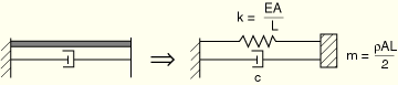
A DASHPOTA element introduces a damping force between two degrees of freedom without introducing any stiffness between these degrees of freedom and without introducing any mass at the nodes. This can cause a reduction in the stable time increment. For example, consider a simple system of a truss element and a dashpot element as shown in Figure 26.2.1–1.

Figure 26.2.1–1 A simple truss and dashpot system.

The dynamic equation for this system is

where

and

The stable time increment for the spring-dashpot system is

As the dashpot coefficient c is increased, the stable time increment,

, will be reduced.

To avoid this reduction in the stable time increment, dashpots should be used in parallel with spring or truss elements, where the stiffness of the spring or truss elements is chosen so that the stable time increment of the dashpot and spring or truss is larger than the stable critical time increment that is calculated by ABAQUS/Explicit. If this requires springs or trusses that have unacceptable forces, specify the time increment size directly for the step (see “Explicit dynamic analysis,” Section 6.3.3).

Relative velocity definition

The relative velocity definition depends on the element type.

DASHPOT1 elements

The relative velocity across a DASHPOT1 element is the ith component of velocity of the dashpot's node:

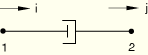
where i is defined as described below and can be in a local direction (see “Defining the direction of action for DASHPOT1 and DASHPOT2 elements”).

DASHPOT2 elements

The relative velocity across a DASHPOT2 element is the difference between the ith component of velocity at the dashpot's first node and the jth component of velocity of the dashpot's second node:

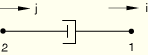
where i and j are defined as described below and can be in local directions (see “Defining the direction of action for DASHPOT1 and DASHPOT2 elements”).

It is important to understand how the DASHPOT2 element will behave according to the above relative displacement equation since the element can produce counterintuitive results. For example, a DASHPOT2 element set up in the following way will be a “compressive” dashpot:

If the nodes have velocities such that and , the dashpot is compressed while the force in the dashpot is positive. To obtain a “tensile” dashpot, the DASHPOT2 element should be set up in the following way:

DASHPOTA elements

The relative velocity across a DASHPOTA element is the difference between the velocity of the dashpot's second node and the dashpot's first node, taken in the direction of the current axis of the dashpot.

For geometrically linear analysis,

where

is the reference position of the dashpot's first node,

is the reference position of the dashpot's second node, and

is the reference length of the dashpot.

For geometrically nonlinear analysis,

where

is the current position of the dashpot's first node,

is the current position of the dashpot's second node, and l is the current length of the dashpot.

In either case the force in a DASHPOTA element is positive if the dashpot is extending.

Defining dashpot behavior

The dashpot behavior can be linear or nonlinear. In either case you must associate the dashpot behavior with a region of your model.

Input File Usage:	DASHPOT, ELSET=name*
	where the ELSET parameter refers to a set of dashpot elements.

ABAQUS/CAE Usage:

Property or Interaction module: SpecialSprings/DashpotsCreate: select connectivity type: select points

Linear dashpot behavior

You define linear dashpot behavior by specifying a constant dashpot coefficient (force per relative velocity).

The dashpot coefficient can depend on temperature and field variables. See “Input syntax rules,” Section 1.2.1, for further information about defining data as functions of temperature and independent field variables.

For direct-solution steady-state dynamic analysis the dashpot coefficient can depend on frequency, as well as on temperature and field variables. If a frequency-dependent dashpot coefficient is specified for any other analysis procedure in ABAQUS/Standard, the data for the lowest frequency given will be used.

Input File Usage:

*DASHPOT, DEPENDENCIES=n
first data line
dashpot coefficient, frequency, temperature, field variable 1, etc.
...

ABAQUS/CAE Usage:	Property or Interaction module: SpecialSprings/DashpotsCreate: select connectivity type: select points: Property: Dashpot coefficient: dashpot coefficient
	Defining the dashpot coefficient as a function of frequency, temperature, and field variables is not supported in ABAQUS/CAE when you define dashpots as engineering features; instead, you can define connectors that have dashpot-like damping behavior (see “Connector damping behavior,” Section 25.2.3).

Nonlinear dashpot behavior

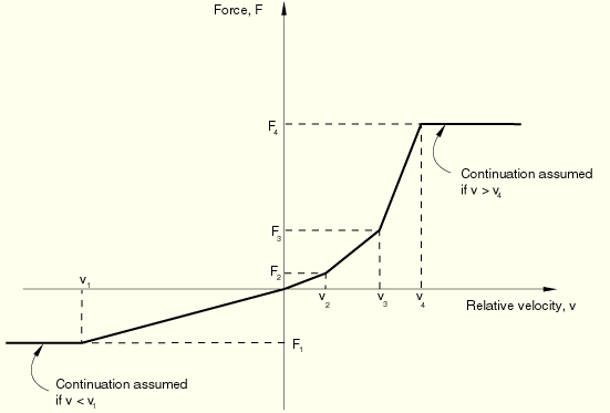
You define nonlinear dashpot behavior by giving pairs of force–relative velocity values. These values should be given in ascending order of relative velocity and should be provided over a sufficiently wide range of relative velocity values so that the behavior is defined correctly. ABAQUS assumes that the force remains constant outside the range given (see Figure 26.2.1–2). In addition, the curve should pass through the origin. That is, the force should be zero at zero relative velocity.

Figure 26.2.1–2 Nonlinear dashpot force-relative velocity relationship.

ABAQUS/Explicit will regularize the data into tables that are defined in terms of even intervals of the independent variables. In some cases where the force is defined at uneven intervals of the independent variable (relative velocity) and the range of the independent variable is large compared to the smallest interval, ABAQUS/Explicit may fail to obtain an accurate regularization of your data in a reasonable number of intervals. In this case the program will stop after all data are processed with an error message that you must redefine the material data. See “Material data definition,” Section 16.1.2, for a more detailed discussion of data regularization.

Input File Usage:

*DASHPOT, NONLINEAR, DEPENDENCIES=n
first data line
force, relative velocity, temperature, field variable 1, etc.
...

ABAQUS/CAE Usage:

Defining nonlinear dashpot behavior is not supported in ABAQUS/CAE when you define dashpots as engineering features; instead, you can define connectors that have dashpot-like damping behavior (see “Connector damping behavior,” Section 25.2.3).

Defining the direction of action for DASHPOT1 and DASHPOT2 elements

You define the direction of action for DASHPOT1 and DASHPOT2 elements by giving the degree of freedom at each node of the element. This degree of freedom may be in a local coordinate system (“Orientations,” Section 2.2.5). This local system is assumed to be fixed: even in large-displacement analysis DASHPOT1 and DASHPOT2 elements act in a fixed direction throughout the analysis.

Input File Usage:

*DASHPOT, ORIENTATION=name
dof at node 1, dof at node 2

ABAQUS/CAE Usage:

Property or Interaction module: SpecialSprings/DashpotsCreate, then select one of the following:
Connect points to ground: select points: Orientation: Edit:
select orientation
Connect two points: select points: Axis: Specify fixed direction:
Orientation: Edit: select orientation

Dashpots within substructures

Dashpots cannot be used within substructures. You can define Rayleigh damping within the substructure definition or on the usage level to create damping within a substructure; see “Defining damping” in “Using substructures,” Section 10.1.1, for more information.