Products: ABAQUS/Standard ABAQUS/Explicit ABAQUS/CAE
The connection-type library contains:
translational basic connection components, which affect translational degrees of freedom at both nodes and may affect rotational degrees of freedom at the first node or at both nodes on the connector element;
rotational basic connection components, which affect only rotational degrees of freedom at both nodes on the connector element;
specialized rotational basic connection components, which in addition to rotational degrees of freedom affect other degrees of freedom at the nodes on the connector element;
assembled connections, which are predefined combinations of translational and rotational or translational and specialized rotational basic connection components; and
complex connections, which affect a combination of degrees of freedom at the nodes on the connector element and cannot be combined with any other connection component.
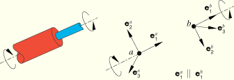
Each connection type is described in the connection-type library. Each library entry includes a figure, which relates the physical behavior to the idealized model and defines the local coordinate directions. Following the figure, each library entry defines kinematic constraints; constraint forces and moments internal to the connection; components of relative motion available for defining the connector behavior, connector motion, or connector loads (called available components); and kinetic forces and moments conjugate to the available components of relative motion. If appropriate, a discussion of the predicted Coulomb-like friction in the connection is included. Finally, the connection type is summarized in a table.
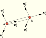
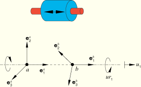
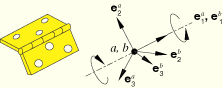
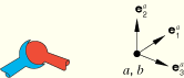
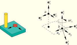
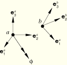
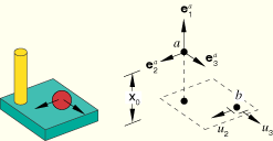
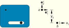
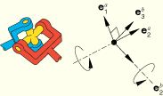
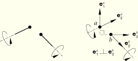
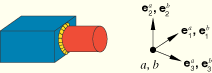
A schematic drawing of each connection type is included along with the ABAQUS idealization of the connection. The idealization indicates in what sense available components of relative motion are measured and how the nodes' positions and orientation directions define the connection. When orientation directions are used to define the connection, the idealization shows these local directions at the appropriate nodes. If available components of relative motion exist in the connection, they are indicated in the figure as free relative motions. For example, the REVOLUTE connection type affects only rotations. It has one available component (the rotation about the shared axis), requires an orientation at node a, and allows an optional orientation at node b.
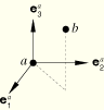
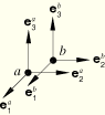
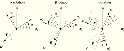
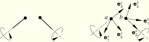
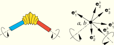
The orientation directions at node a (the first node on the connector element) are indicated as unit base vectors ![]() , where
, where ![]() . Similarly, the orientation directions at node b are indicated as
. Similarly, the orientation directions at node b are indicated as ![]() . When orientation directions are required at a node, you must define them as described in “Orientations,” Section 2.2.5. If orientation directions are optional but not provided at node a, the global directions are used by default. If orientation directions are optional but not provided at node b, the orientation directions from node a are used by default.
. When orientation directions are required at a node, you must define them as described in “Orientations,” Section 2.2.5. If orientation directions are optional but not provided at node a, the global directions are used by default. If orientation directions are optional but not provided at node b, the orientation directions from node a are used by default.
Connector elements activate rotational degrees of freedom at the nodes to which they are attached if they do not exist already and an orientation is permitted at that node. The only exception is connection type JOIN, where an orientation is optional at node a but rotation degrees of freedom are not activated.
The orientation directions co-rotate with the rotation of the node to which they are attached (with the exception of connection type JOIN, which uses fixed directions when rotation degrees of freedom are not active at node a). If there are no elements with rotational degrees of freedom attached to the node, rotational multi-point constraints, or rotational equations, you must ensure that sufficient rotational boundary conditions are provided to avoid numerical singularities associated with unconstrained rotational degrees of freedom.
The six components of relative motion, denoted ![]() and
and ![]() for
for ![]() , are defined in the description for each connection, where needed. These components include constrained and available components of relative motion. Forces and moments are denoted
, are defined in the description for each connection, where needed. These components include constrained and available components of relative motion. Forces and moments are denoted ![]() and
and ![]() . These quantities are either constraint forces and moments, which enforce the kinematic constraints on the constrained components of relative motion, or kinetic forces and moments, which are the work conjugate variables to the available components of relative motion. For example, the REVOLUTE connection type has one available component of relative motion,
. These quantities are either constraint forces and moments, which enforce the kinematic constraints on the constrained components of relative motion, or kinetic forces and moments, which are the work conjugate variables to the available components of relative motion. For example, the REVOLUTE connection type has one available component of relative motion, ![]() , and two kinematic rotation constraints (equivalent to setting two rotation components,
, and two kinematic rotation constraints (equivalent to setting two rotation components, ![]() and
and ![]() , to zero). Conjugate to the available rotation component is the kinetic moment
, to zero). Conjugate to the available rotation component is the kinetic moment ![]() acting about the local
acting about the local ![]() -direction.
-direction.
In general, kinetic forces and moments include the effects of connector behaviors, such as elastic springs, viscous damping, friction, and reaction forces and moments due to connector stops and locks. For constitutive response defined as a function of displacement or rotation, the initial position may not correspond with the reference position where constitutive forces and moments are zero. You can define reference lengths and angles (given in degrees) for connector behavior as described in “Defining reference lengths and angles for constitutive response” in “Connector behavior,” Section 25.2.1. These reference quantities define ![]() and
and ![]() , the connector constitutive displacements and rotations. These constitutive displacements and rotations are used only to define constitutive response and differ from the relative displacements and rotations measured in the connector elements only when you define the reference lengths or angles.
, the connector constitutive displacements and rotations. These constitutive displacements and rotations are used only to define constitutive response and differ from the relative displacements and rotations measured in the connector elements only when you define the reference lengths or angles.
As an example, if the REVOLUTE connection included linear spring and dashpot behavior combined with a connector stop,
![]()
Coulomb-like friction behavior is possible for any connection type that has available components of relative motion; see “Connector friction behavior,” Section 25.2.5, for details. Friction behavior requires a “tangent” direction (the direction in which slipping may occur) and a “normal” direction (the direction perpendicular to the contacting surfaces). In the most general case you define the normal force causing friction in the connector. However, ABAQUS predefines friction behavior for a limited number of connection types, as discussed in the connection-type library in this section. In these predefined friction cases you do not have to define the contact normal force.
Each connection library entry includes a table summarizing the connection type. This summary table indicates whether the connection type is basic or assembled. It gives the kinematic constraints; constraint force or moment components; available components of relative motion; “kinetic” force or moment components following from the constitutive behavior in the available components of relative motion; which orientation directions are required, optional, or ignored; how connector stops limit the available components of relative motion; what reference lengths and angles are used to define the constitutive behavior; what parameters are used for predefined Coulomb-like friction; and how the contact normal forces are defined by ABAQUS in association with predefined Coulomb-like friction.
Basic connection components are divided into three categories:
Translational basic connection components, which affect translational degrees of freedom at both nodes and may affect rotational degrees of freedom at the first node or at both nodes
Rotational basic connection components, which affect only rotational degrees of freedom at both nodes
Specialized rotational basic connection components, which in addition to rotational degrees of freedom affect other degrees of freedom at the nodes
The following basic connection components affect translational degrees of freedom at both node a and node b. Some of these connector components affect rotational degrees of freedom at node a or at both node a and node b. Any basic connection component from this list can be used to define the translational behavior of a connector element.
ACCELEROMETER Provide a connection between two nodes to measure the relative acceleration, velocity, and position of a body in a local coordinate system. This connection type is available only in ABAQUS/Explicit. If it is defined in an ABAQUS/Standard model, it will be converted internally to a CARTESIAN connector type.
AXIAL Provide a connection between two nodes that acts along the line connecting the nodes.
CARTESIAN Provide a connection between two nodes that allows independent behavior in three local Cartesian directions that follow the system at node a.
JOIN Join the position of two nodes.
LINK Provide a pinned rigid link between two nodes to keep the distance between the two nodes constant.
PROJECTION CARTESIAN Provide a connection between two nodes that allows independent behavior in three local Cartesian directions that follow the system at both nodes a and b.
RADIAL-THRUST Provide a connection between two nodes that allows different behavior for radial and thrust displacements.
SLIDE-PLANE Provide a slide-plane connection to make the position of the second node remain on a plane defined by the orientation of the first node and the initial position of the second node.
SLOT Provide a slot connection to make the position of the second node remain on a line defined by the orientation of the first node and the initial position of the second node.
The following basic connection components affect only rotational degrees of freedom at the nodes in the connection. Any basic connection component from this list can be used to define the rotational behavior of a connector element.
ALIGN Provide a connection between two nodes that aligns their local directions.
CARDAN Provide a rotational connection between two nodes parameterized by Cardan (or Bryant) angles.
CONSTANT VELOCITY Provide a constant velocity connection between two nodes.
EULER Provide a rotational connection between two nodes parameterized by Euler angles.
FLEXION-TORSION Provide a connection between two nodes that allows different behavior for flexural and torsional rotations.
PROJECTION FLEXION-TORSION Provide a connection between two nodes that allows different behavior for two flexural rotations and one torsional rotation.
REVOLUTE Provide a revolute connection between two nodes.
ROTATION Provide a rotational connection between two nodes parameterized by the rotation vector.
ROTATION-ACCELEROMETER Provide a connection between two nodes to measure the relative angular acceleration, velocity, and position of a body in a local coordinate system. This connection type is available only in ABAQUS/Explicit. If it is defined in an ABAQUS/Standard model, it will be converted internally to a CARDAN connector type.
UNIVERSAL Provide a universal connection between two nodes.
The following basic connection component affects rotational and other non-translational degrees of freedom at the nodes in the connection. The specialized rotational basic connection component can be combined with translational basic connection components.
FLOW-CONVERTER Provide a means of converting the material flow (degree of freedom 10) at a connector node into a rotation.
Assembled connections are included for convenience. Each assembled connection is created by combinations of basic connection components. The equivalent basic connection components used for each assembled connection are listed in parentheses.
BEAM Provide a rigid beam connection between two nodes. (JOIN + ALIGN)
BUSHING Provide a connection between two nodes that allows independent behavior in three local Cartesian directions that follow the system at both nodes a and b and that allows different behavior in two flexural rotations and one torsional rotation. (PROJECTION CARTESIAN + PROJECTION FLEXION-TORSION)
CVJOINT Join the position of two nodes, and provide a constant velocity connection between their rotational degrees of freedom. (JOIN + CONSTANT VELOCITY)
CYLINDRICAL Provide a slot connection between two nodes, and constrain the rotations by a revolute connection. (SLOT + REVOLUTE)
HINGE Join the position of two nodes, and provide a revolute connection between their rotational degrees of freedom. (JOIN + REVOLUTE)
PLANAR Provide a slide-plane connection between two nodes with a revolute connection about the normal direction to the plane. The PLANAR connection creates a local two-dimensional system in three-dimensional analyses. (SLIDE-PLANE + REVOLUTE)
RETRACTOR Join the position of two nodes, and convert material flow into rotation. (JOIN + FLOW-CONVERTER)
TRANSLATOR Provide a slot connection between two nodes, and align their three local axis directions. (SLOT + ALIGN)
UJOINT Join the position of two nodes, and provide a universal connection between their rotational degrees of freedom at the nodes. (JOIN + UNIVERSAL)
WELD Join the position of two nodes, and align their three local axis directions. (JOIN + ALIGN)
Complex connections affect a combination of degrees of freedom at the nodes in the connection and cannot be combined with other connection components. They typically model highly coupled physical connections.
SLIPRING Model material flow and stretching between two points of a belt system (such as an automotive seat belt).
The following descriptions list all the basic connection components and assembled connections in alphabetical order.
Connection type ACCELEROMETER provides a convenient way to measure the relative position, velocity, and acceleration of a body in a local coordinate system. These kinematic quantities are measured relative to the motion of node a and are reported in the coordinate system of node b. Each node of the connector can translate and rotate independently, although fixing the first of the two nodes to ground is more common. With the first node fixed, connection type ACCELEROMETER provides a convenient way to measure the local components of the velocity and acceleration in a coordinate system fixed to a moving body (for example, an accelerometer).
Connection type ACCELEROMETER is available only in ABAQUS/Explicit. It is the translation counterpart to connection type ROTATION-ACCELEROMETER, which measures relative angular position, velocity, and acceleration. ACCELEROMETER connectors cannot be used in two-dimensional and axi-symmetric analysis in ABAQUS/Explicit.
The ACCELEROMETER connection does not impose kinematic constraints. It defines three local directions at node a and three local directions at node b. The ACCELEROMETER connection's formulation is similar to that for the CARTESIAN connection. The ACCELEROMETER connection measures the position of node b relative to node a
![]()
![]()
The ACCELEROMETER connection measures velocity and acceleration in the local directions at node a as if node a were an inertial frame. In contrast to the CARTESIAN connection, the ACCELEROMETER connection reports the computed velocity and acceleration in the local directions at node b. Let ![]() be the transformation from
be the transformation from ![]() to
to ![]() . Then the ACCELEROMETER connection measures velocity and acceleration as
. Then the ACCELEROMETER connection measures velocity and acceleration as
![]()
In two-dimensional and axisymmetric analyses ![]() .
.
| ACCELEROMETER | |
|---|---|
| Basic or assembled: | Basic |
| Kinematic constraints: | None |
| Constraint force output: | None |
| Available components: | None |
| Kinetic force output: | None |
| Orientation at a: | Optional |
| Orientation at b: | Optional |
| Connector stops: | None |
| Constitutive reference lengths: | None |
| Predefined friction parameters: | None |
| Contact force for predefined friction: | None |
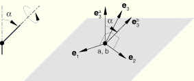
Connection type ALIGN provides a connection between two nodes where all three local directions are aligned. If both local axes are given and do not align initially, their initial relative angular position is held constant.
The ALIGN connection imposes kinematic constraints only. The local directions at node b are set equal to those at node a. If the local directions do not align initially, the ALIGN connection holds fixed the Cardan angles between the local orientation directions at node b, ![]() , and those at node a,
, and those at node a, ![]() . These fixed angular positions are the connector position output quantities. See connection type CARDAN for a definition of Cardan angles.
. These fixed angular positions are the connector position output quantities. See connection type CARDAN for a definition of Cardan angles.
The constraint moment enforcing the alignment of the local directions is
![]()
| ALIGN | |
|---|---|
| Basic or assembled: | Basic |
| Kinematic constraints: | |
| Constraint moment output: | |
| Available components: | None |
| Kinetic moment output: | None |
| Orientation at a: | Optional |
| Orientation at b: | Optional |
| Connector stops: | None |
| Constitutive reference angles: | None |
| Predefined friction parameters: | None |
| Contact force for predefined friction: | None |
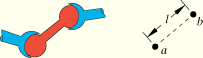
Connection type AXIAL provides a connection between two nodes where the relative displacement is along the line separating the two nodes. It models discrete physical connections such as axial springs, axial dashpots, or node-to-node (gap-like) contact.
The AXIAL connection does not constrain any component of relative motion. The distance between nodes a and b is
![]()
![]()
![]()
The kinetic force is
![]()
An optional orientation can be provided at one of the nodes in an AXIAL connection to provide direction for the force if the nodes are coincident or when one of the nodes is a “ground node.” If the orientation is provided at both of the coincident nodes, the orientation at the first node in the connectivity will be used. The orientation definitions will be ignored when the two nodes separate. Rotational degrees of freedom are not activated for connection type AXIAL.
Connection type BEAM provides a rigid beam connection between two nodes.
Connection type BEAM imposes kinematic constraints and uses local orientation definitions equivalent to combining connection types JOIN and ALIGN.
| BEAM | |
|---|---|
| Basic or assembled: | Assembled |
| Kinematic constraints: | JOIN + ALIGN |
| Constraint force and moment output: | |
| Available components: | None |
| Kinetic force and moment output: | None |
| Orientation at a: | Optional |
| Orientation at b: | Optional |
| Connector stops: | None |
| Constitutive reference lengths and angles: | None |
| Predefined friction parameters: | None |
| Contact force for predefined friction: | None |
Connection type BUSHING provides a bushing-like connection between two nodes. It cannot be used in two-dimensional or axisymmetric analyses.
Connection type BUSHING does not constrain any components of relative motion and uses local orientation definitions equivalent to combining connection types PROJECTION CARTESIAN and PROJECTION FLEXION-TORSION.
| BUSHING | |
|---|---|
| Basic or assembled: | Assembled |
| Kinematic constraints: | None |
| Constraint force and moment output: | None |
| Available components: | |
| Kinetic force and moment output: | |
| Orientation at a: | Required |
| Orientation at b: | Optional |
| Connector stops: | |
| Constitutive reference lengths and angles: | |
| Predefined friction parameters: | None |
| Contact force for predefined friction: | None |
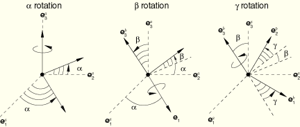
Connection type CARDAN provides a rotational connection between two nodes where the relative rotation between the nodes is parameterized by Cardan (or Bryant) angles. A Cardan-angle parameterization of finite rotations is also called a 1–2–3 or yaw-pitch-roll parameterization. Connection type CARDAN cannot be used in two-dimensional or axisymmetric analysis.
When connection type CARDAN is used with connector behavior, the relative rotation axis with the highest resistance to rotational motion should be assigned to the second component of relative rotation (component number 5) to avoid “gimbal lock,” a singularity in the rotation parameterization for relative rotation angles ![]() .
.
The CARDAN connection does not impose kinematic constraints. A CARDAN connection is a finite rotation connection where the local directions at node b are parameterized in terms of Cardan (or Bryant) angles relative to the local directions at node a. Local directions ![]() are positioned relative to
are positioned relative to ![]() by three successive finite rotations
by three successive finite rotations ![]() ,
, ![]() , and
, and ![]() as follows:
as follows:
Rotate by ![]() radians about axis
radians about axis ![]() ;
;
Rotate by ![]() radians about the intermediate 2-axis,
radians about the intermediate 2-axis, ![]() ; and
; and
Rotate by ![]() radians about axis
radians about axis ![]() .
.
![]()
![]()
![]()
The three available components of relative motion in the CARDAN connection are the changes in the Cardan angles positioning the local directions at node b relative to the local directions at node a. Therefore,
![]()
![]()
The kinetic moment in a CARDAN connection is determined from the three component relationships:
![]()
| CARDAN | |
|---|---|
| Basic or assembled: | Basic |
| Kinematic constraints: | None |
| Constraint moment output: | None |
| Available components: | |
| Kinetic moment output: | |
| Orientation at a: | Required |
| Orientation at b: | Optional |
| Connector stops: | |
| Constitutive reference angles: | |
| Predefined friction parameters: | None |
| Contact force for predefined friction: | None |
Connection type CARTESIAN provides a connection between two nodes where the response in three local connection directions is specified.
The CARTESIAN connection does not impose kinematic constraints. It defines three local directions ![]() at node a and measures the change in position of node b along these local coordinate directions. The local directions at node a follow the rotation of node a.
at node a and measures the change in position of node b along these local coordinate directions. The local directions at node a follow the rotation of node a.
The position of node b relative to node a is
![]()
![]()
![]()
The kinetic force is
![]()
In two-dimensional analysis ![]() ,
, ![]() ,
, ![]() , and
, and ![]() .
.
| CARTESIAN | |
|---|---|
| Basic or assembled: | Basic |
| Kinematic constraints: | None |
| Constraint force output: | None |
| Available components: | |
| Kinetic force output: | |
| Orientation at a: | Optional |
| Orientation at b: | Ignored |
| Connector stops: | |
| Constitutive reference lengths: | |
| Predefined friction parameters: | None |
| Contact force for predefined friction: | None |
Connection type CONSTANT VELOCITY provides the rotational part of a constant velocity joint. It cannot be used in two-dimensional or axisymmetric analysis. Furthermore, the connection type does not have available components of relative motion. To include connector behavior in flexural motion, use connection type FLEXION-TORSION with the torsion angle set to zero.
This connection type models physical connectors that under certain conditions transmit a constant spinning velocity about misaligned shafts.
The shaft direction at node a is ![]() , and the shaft direction at node b is
, and the shaft direction at node b is ![]() . The constant velocity constraint is stated as follows. In any configuration there are two unit length orthogonal vectors
. The constant velocity constraint is stated as follows. In any configuration there are two unit length orthogonal vectors ![]() and
and ![]() in the plane perpendicular to the shaft at node b. These vectors can be written
in the plane perpendicular to the shaft at node b. These vectors can be written
![]()
![]()
The name “constant velocity” for this connection type derives from the following property. If the angular velocities of the two shafts, ![]() and
and ![]() , have components only along each shaft, respectively, and in the direction of the normal to the plane containing the two shafts (that is, along the
, have components only along each shaft, respectively, and in the direction of the normal to the plane containing the two shafts (that is, along the ![]() direction), the components of angular velocity along the respective shaft directions are equal:
direction), the components of angular velocity along the respective shaft directions are equal:
![]()
The constraint moment imposing the constant velocity constraint has a single component about the average shaft direction ![]() and is written
and is written
![]()
| CONSTANT VELOCITY | |
|---|---|
| Basic or assembled: | Basic |
| Kinematic constraints: | |
| Constraint moment output: | |
| Available components: | None |
| Kinetic moment output: | None |
| Orientation at a: | Required |
| Orientation at b: | Optional |
| Connector stops: | None |
| Constitutive reference angles: | None |
| Predefined friction parameters: | None |
| Contact force for predefined friction: | None |
Connection type CVJOINT joins the position of two nodes and provides a constant velocity constraint between their rotational degrees of freedom. Connection type CVJOINT cannot be used in two-dimensional or axisymmetric analysis.
Connection type CVJOINT imposes kinematic constraints and uses local orientation definitions equivalent to combining connection types JOIN and CONSTANT VELOCITY.
| CVJOINT | |
|---|---|
| Basic or assembled: | Assembled |
| Kinematic constraints: | JOIN + CONSTANT VELOCITY |
| Constraint force and moment output: | |
| Available components: | None |
| Kinetic force and moment output: | None |
| Orientation at a: | Required |
| Orientation at b: | Optional |
| Connector stops: | None |
| Constitutive reference lengths and angles: | None |
| Predefined friction parameters: | None |
| Contact force for predefined friction: | None |
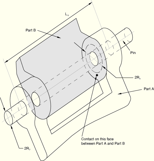
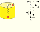
Connection type CYLINDRICAL provides a slot connection between two nodes and a revolute constraint where the free rotation is about the line of the slot. It cannot be used in two-dimensional or axisymmetric analysis.
Connection type CYLINDRICAL imposes kinematic constraints and uses local orientation definitions equivalent to combining connection types SLOT and REVOLUTE.
The connector constraint forces and moments reported as connector output depend strongly on the order and the location of the nodes in the connector (see “Connector behavior,” Section 25.2.1). Since the kinematic constraints are enforced at node b (the second node of the connector element), the reported forces and moments are the constraint forces and moments applied at node b to enforce the CYLINDRICAL constraint. Thus, in most cases the connector output associated with a CYLINDRICAL connection is best interpreted when node b is located at the center of the device enforcing the constraint. This choice is essential when moment-based friction is modeled in the connector since the contact forces are derived on the connector forces and moments, as illustrated below. Proper enforcement of the kinematic constraints is independent of the order or location of the nodes.
Predefined Coulomb-like friction in the CYLINDRICAL connection defines the friction force (CSFC) along the instantaneous slip direction on the two contacting cylindrical surfaces (the pin and the sleeve) illustrated above. The table below summarizes the parameters that are used to specify predefined friction in this connection type as discussed in detail next.
The frictional effect is formally written as
![]()
The normal force ![]() is the sum of a magnitude measure of contact friction-producing connector forces,
is the sum of a magnitude measure of contact friction-producing connector forces, ![]() , and a self-equilibrated internal contact force (such as from a press-fit assembly),
, and a self-equilibrated internal contact force (such as from a press-fit assembly), ![]() :
:
![]()
The contact force magnitude ![]() is defined by summing the following two contributions:
is defined by summing the following two contributions:
a radial force contribution, ![]() (the magnitude of the constraint forces enforcing the SLOT constraint):
(the magnitude of the constraint forces enforcing the SLOT constraint):
![]()
a force contribution from “bending,” ![]() , obtained by scaling the bending moment,
, obtained by scaling the bending moment, ![]() (the magnitude of the constraint moments enforcing the REVOLUTE constraint), by a length factor, as follows:
(the magnitude of the constraint moments enforcing the REVOLUTE constraint), by a length factor, as follows:
![]()
![]()
![]()
The magnitude of the frictional tangential tractions, ![]() is computed using
is computed using
![]()
| CYLINDRICAL | |
|---|---|
| Basic or assembled: | Assembled |
| Kinematic constraints: | SLOT + REVOLUTE |
| Constraint force and moment output: | |
| Available components: | |
| Kinetic force and moment output: | |
| Orientation at a: | Required |
| Orientation at b: | Optional |
| Connector stops: | |
| Constitutive reference lengths and angles: | |
| Predefined friction parameters: | Required: R; optional: L, |
| Contact force for predefined friction: | |
Connection type EULER provides a rotational connection between two nodes where the total relative rotation between the nodes is parameterized by Euler angles. An Euler-angle parameterization of finite rotations is also called a 3–1–3 or precession-nutation-spin parameterization. Connection type EULER cannot be used in two-dimensional or axisymmetric analysis.
The EULER connection does not impose kinematic constraints. An EULER connection is a finite rotation connection where the local directions at node b are parameterized in terms of Euler angles relative to the local directions at node a. Local directions ![]() are positioned relative to
are positioned relative to ![]() by three successive finite rotations
by three successive finite rotations ![]() ,
, ![]() , and
, and ![]() as follows:
as follows:
Rotate by ![]() radians about axis
radians about axis ![]() ;
;
Rotate by ![]() radians about the intermediate 1-axis,
radians about the intermediate 1-axis, ![]() ;
;
Rotate by ![]() radians about axis
radians about axis ![]() .
.
![]()
![]()
![]()
If the intermediate rotation is an even multiple of ![]() ,
, ![]() , where
, where ![]() , the other two Euler angles become non-unique. In this case
, the other two Euler angles become non-unique. In this case
![]()
![]()
The available components of relative motion in the EULER connection are the changes in the Euler angles that position the local directions at node b relative to the local directions at node a. Therefore,
![]()
![]()
The kinetic moment in a EULER connection is determined from the three component relationships:
![]()
| EULER | |
|---|---|
| Basic or assembled: | Basic |
| Kinematic constraints: | None |
| Constraint moment output: | None |
| Available components: | |
| Kinetic moment output: | |
| Orientation at a: | Required |
| Orientation at b: | Optional |
| Connector stops: | |
| Constitutive reference angles: | |
| Predefined friction parameters: | None |
| Contact force for predefined friction: | None |
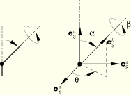
Connection type FLEXION-TORSION provides a rotational connection between two nodes. It models the bending and twisting of a cylindrical coupling between two shafts. In this case the response to twist rotations about the shafts may differ from the response to bending of the shafts. Connection type FLEXION-TORSION cannot be used in two-dimensional or axisymmetric analysis.
The flexural part of the connection resists bending misalignment of the two shafts, whereas the torsional part of the connection resists relative rotations about the shafts. Connection type FLEXION-TORSION can be used in conjunction with connection type RADIAL-THRUST when resistance to relative radial and thrust displacements is modeled.
The FLEXION-TORSION connection does not impose kinematic constraints. The FLEXION-TORSION connection describes a finite rotation by three angles: flexion, torsion, and sweep (![]() ,
, ![]() , and
, and ![]() ). However, the flexion, torsion, and sweep angles do not represent three successive rotations. The flexion angle between two shafts measures the angle of misalignment of the two shafts and is always reported as a positive angle. The torsion angle measures the twist of one shaft relative to the other.
). However, the flexion, torsion, and sweep angles do not represent three successive rotations. The flexion angle between two shafts measures the angle of misalignment of the two shafts and is always reported as a positive angle. The torsion angle measures the twist of one shaft relative to the other.
The sweep angle orients the rotation vector, in the ![]() –
–![]() plane, for the flexion motion. See Figure 25.1.5–13. Since the flexion angle is never negative, the sweep angle may undergo discontinuous jumps by up to
plane, for the flexion motion. See Figure 25.1.5–13. Since the flexion angle is never negative, the sweep angle may undergo discontinuous jumps by up to ![]() radians when the flexion angle passes through zero. An analysis may give inaccurate results or may not converge if any jump occurs in the sweep angle. In general, the sweep angle is not used as an available component of relative motion for which connector behavior is defined. Rather, it is used to define angular dependence for the elastic constitutive response in flexion deformations (as an independent component in the connector elastic behavior definition). Since the sweep angle is restricted to the interval
radians when the flexion angle passes through zero. An analysis may give inaccurate results or may not converge if any jump occurs in the sweep angle. In general, the sweep angle is not used as an available component of relative motion for which connector behavior is defined. Rather, it is used to define angular dependence for the elastic constitutive response in flexion deformations (as an independent component in the connector elastic behavior definition). Since the sweep angle is restricted to the interval ![]() to
to ![]() radians, any dependence on the sweep angle should be periodic, such that the behavior for
radians, any dependence on the sweep angle should be periodic, such that the behavior for ![]() is the same as
is the same as ![]() . Since
. Since ![]() is a singular point for which the sweep angle is not uniquely defined, it is strongly recommended that any connector behavior that defines flexural moment versus flexion angle gives zero moment at zero flexion angle. If connector behavior is defined in the sweep available component, the sweep moment must be zero at flexion angles
is a singular point for which the sweep angle is not uniquely defined, it is strongly recommended that any connector behavior that defines flexural moment versus flexion angle gives zero moment at zero flexion angle. If connector behavior is defined in the sweep available component, the sweep moment must be zero at flexion angles ![]() and
and ![]() .
.
The FLEXION-TORSION connection is similar to a finite successive rotation parameterization 3–2–3. However, in terms of the 3–2–3 parameterization, the sweep angle is the first rotation angle, the flexion angle is the second rotation angle, and the torsion angle is the sum of the first and third rotation angles.
The first shaft direction at node a is ![]() , and the second shaft direction at node b is
, and the second shaft direction at node b is ![]() . Let the two shafts form an angle
. Let the two shafts form an angle ![]() , called the flexion angle. Then,
, called the flexion angle. Then,
![]()
![]()
![]()
The sweep angle ![]() measures the angle from
measures the angle from ![]() to the projection of
to the projection of ![]() onto the
onto the ![]() –
–![]() plane. With this definition
plane. With this definition
![]()
![]()
A singularity in the definition of the sweep angles occurs when the flexion angle ![]() vanishes. In this case
vanishes. In this case ![]() ; that is, the torsion and sweep angle axes are coincident, and the two angles are no longer independent. When
; that is, the torsion and sweep angle axes are coincident, and the two angles are no longer independent. When ![]() , the sweep angle is assumed zero,
, the sweep angle is assumed zero, ![]() .
.
The available components of relative motion ![]() ,
, ![]() , and
, and ![]() are the changes in the flexion, torsion, and sweep angles and are defined as
are the changes in the flexion, torsion, and sweep angles and are defined as
![]()
![]()
The kinetic moment in a FLEXION-TORSION connection is determined from the three component relationships:
![]()
| FLEXION-TORSION | |
|---|---|
| Basic or assembled: | Basic |
| Kinematic constraints: | None |
| Constraint moment output: | None |
| Available components: | |
| Kinetic moment output: | |
| Orientation at a: | Required |
| Orientation at b: | Optional |
| Connector stops: | |
| Constitutive reference angles: | |
| Predefined friction parameters: | None |
| Contact force for predefined friction: | None |
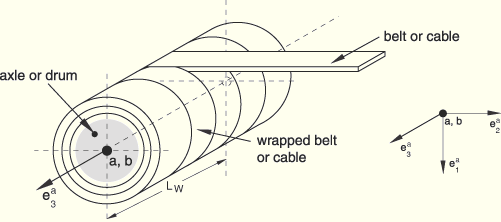
Connection type FLOW-CONVERTER converts the material flow degree of freedom (10) at the second node of a connector element into a rotation about a user-specified axis at the first node of the connector. This connection type can be used to model retractor and pretensioner devices in automotive seat belts (see “Seat belt analysis of a simplified crash dummy,” Section 3.3.1 of the ABAQUS Example Problems Manual) or cable drums in winch-like devices. Belt or cable material is considered to be wrapped around an axle or a drum, and material can be spooled either into or out of the connector element.
This connection type activates degree of freedom 10 at the second node of a connector. As with any other nodal degree of freedom, you must be careful in constraining it. This is typically done by attaching the connector to a SLIPRING connector that is part of the belt system or by applying a boundary condition. FLOW-CONVERTER connectors cannot be used in two-dimensional and axi-symmetric analysis in ABAQUS/Explicit.
The FLOW-CONVERTER connection constrains the rotation about the third local direction, ![]() , to the material flow at node b,
, to the material flow at node b, ![]() . The constraint can be written as
. The constraint can be written as
![]()
There are no available components of relative motion for this connection type; hence, kinetic behavior cannot be specified. However, the following kinematic quantities are available for output:
![]()
The constraint moment is
![]()
At most two FLOW-CONVERTER connectors can share their second node where degree of freedom 10 is active.
| FLOW-CONVERTER | |
|---|---|
| Basic or assembled: | Specialized basic rotational |
| Kinematic constraints: | |
| Constraint moment output: | |
| Available components: | None |
| Kinetic force output: | None |
| Orientation at a: | Required |
| Orientation at b: | Ignored |
| Connector stops: | None |
| Constitutive reference lengths: | None |
| Predefined friction parameters: | None |
| Contact force for predefined friction: | None |
Connection type HINGE joins the position of two nodes and provides a revolute constraint between their rotational degrees of freedom. Connection type HINGE cannot be used in two-dimensional or axisymmetric analysis.
Connection type HINGE imposes kinematic constraints and uses local orientation definitions equivalent to combining connection types JOIN and REVOLUTE.
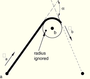
The connector constraint forces and moments reported as connector output depend strongly on the order and the location of the nodes in the connector element (see “Connector behavior,” Section 25.2.1). Since the kinematic constraints are enforced at node b (the second node of the connector element), the reported forces and moments are the constraint forces and moments applied at node b to enforce the HINGE constraint. Thus, in most cases the connector output associated with a HINGE connection is best interpreted when node b is located at the center of the device enforcing the constraint. This choice is essential when moment-based friction is modeled in the connector since the contact forces are derived from the connector forces and moments, as illustrated below. Proper enforcement of the kinematic constraints is independent of the order or location of the nodes.
Predefined Coulomb-like friction in the HINGE connection relates the kinematic constraint forces and moments in the connector to a friction moment (CSM1) in the rotation about the hinge axis. The table below summarizes the parameters that are used to specify predefined friction in this connection type as discussed in detail next. A typical interpretation of the geometric scaling constants is illustrated in Figure 25.1.5–16.
Since the rotation about the 1-direction is the only possible relative motion in the connection, the frictional effect is formally written in terms of moments generated by tangential tractions and moments generated by contact forces, as follows:
![]()
The normal moment ![]() is the sum of a magnitude measure of contact friction-producing connector moments,
is the sum of a magnitude measure of contact friction-producing connector moments, ![]() , and a self-equilibrated internal contact moment (such as from a press-fit assembly),
, and a self-equilibrated internal contact moment (such as from a press-fit assembly), ![]() :
:
![]()
The contact moment magnitude ![]() is defined by summing the following contributions:
is defined by summing the following contributions:
an axial moment contribution, ![]() , where
, where ![]() and
and ![]() is an effective friction arm associated with the constraint force in the axial direction (the
is an effective friction arm associated with the constraint force in the axial direction (the ![]() radius could be interpreted as an average radius of the outer sleeve cylindrical sections as found in a typical door hinge or as an effective radius associated with the hinge end caps, if they exist; if
radius could be interpreted as an average radius of the outer sleeve cylindrical sections as found in a typical door hinge or as an effective radius associated with the hinge end caps, if they exist; if ![]() is 0.0,
is 0.0, ![]() is ignored); and
is ignored); and
a normal moment contribution, ![]() , where
, where ![]() is the radius of the pin cross-section in the local 2–3 plane and
is the radius of the pin cross-section in the local 2–3 plane and ![]() is itself a sum of the following two contributions:
is itself a sum of the following two contributions:
a radial force contribution, ![]() (the magnitude of the constraint forces enforcing the translation constraints in the local 2–3 plane):
(the magnitude of the constraint forces enforcing the translation constraints in the local 2–3 plane):
![]()
a force contribution from “bending,” ![]() , obtained by scaling the bending moment,
, obtained by scaling the bending moment, ![]() (the magnitude of the constraint moments enforcing the REVOLUTE constraint), by a length factor, as follows:
(the magnitude of the constraint moments enforcing the REVOLUTE constraint), by a length factor, as follows:
![]()
![]()
![]()
The moment magnitude of the frictional tangential tractions, ![]() .
.
| HINGE | |
|---|---|
| Basic or assembled: | Assembled |
| Kinematic constraints: | JOIN + REVOLUTE |
| Constraint force and moment output: | |
| Available components: | |
| Kinetic force and moment output: | |
| Orientation at a: | Required |
| Orientation at b: | Optional |
| Connector stops: | |
| Constitutive reference lengths and angles: | |
| Predefined friction parameters: | Required: |
| Contact moment for predefined friction: | |
Connection type JOIN makes the position of two nodes the same. If the two nodes are not co-located initially, the position of node b is fixed relative to that of node a in a Cartesian coordinate system attached to node a.
Even though an orientation is optional at node a, connection type JOIN does not activate rotational degrees of freedom at node a.
The JOIN connection makes the position of node b equal to that of node a. If the two nodes are not coincident initially, the Cartesian coordinates of node b relative to node a are fixed. See connection type CARTESIAN for a definition of the Cartesian coordinates of node b relative to node a. If rotational degrees of freedom exist at node a, the local directions co-rotate with the node.
The constraint force in the JOIN connection acts in the three local directions at node a and is
![]()
When used by itself, there is no predefined Coulomb-like friction in the JOIN connection, since there are no available components of relative motion for which friction can be defined. However, when the JOIN and REVOLUTE connection types are used together, the predefined friction is the same as the HINGE connection. When the JOIN and UNIVERSAL connection types are used together, the predefined friction is the same as the UJOINT connection.
| JOIN | |
|---|---|
| Basic or assembled: | Basic |
| Kinematic constraints: | |
| Constraint force output: | |
| Available components: | None |
| Kinetic force output: | None |
| Orientation at a: | Optional |
| Orientation at b: | Ignored |
| Connector stops: | None |
| Constitutive reference lengths: | None |
| Predefined friction parameters: | None |
| Contact force for predefined friction: | None |
Connection type LINK maintains a constant distance between two nodes. Rotational degrees of freedom, if they exist, are not affected at either node.
The LINK connection constrains the position of node b, ![]() , to a constant distance from node a. The distance between the two nodes is
, to a constant distance from node a. The distance between the two nodes is
![]()
![]()
| LINK | |
|---|---|
| Basic or assembled: | Basic |
| Kinematic constraints: | |
| Constraint force output: | |
| Available components: | None |
| Kinetic force output: | None |
| Orientation at a: | Ignored |
| Orientation at b: | Ignored |
| Connector stops: | None |
| Constitutive reference lengths: | None |
| Predefined friction parameters: | None |
| Contact force for predefined friction: | None |
Connection type PLANAR provides a local two-dimensional system in a three-dimensional analysis. Connection type PLANAR cannot be used in two-dimensional or axisymmetric analysis.
Connection type PLANAR imposes kinematic constraints and uses local orientation definitions equivalent to combining connection types SLIDE-PLANE and REVOLUTE.
Predefined Coulomb-like friction in the PLANAR connection relates the kinematic constraint forces and moments in the connector to the friction forces in the translations in the local 2–3 plane and the rotations about the local 1-direction. These two frictional effects are discussed separately below.
The frictional effect due to sliding in the 2–3 plane is formally written as
![]()
The normal force ![]() is the sum of a magnitude measure of contact force-producing connector forces,
is the sum of a magnitude measure of contact force-producing connector forces, ![]() , and a self-equilibrated internal contact force,
, and a self-equilibrated internal contact force, ![]() :
:
![]()
The contact force magnitude ![]() is defined by summing the following two contributions:
is defined by summing the following two contributions:
a contact force contribution, ![]() (the constraint force enforcing the SLIDE-PLANE constraint); and
(the constraint force enforcing the SLIDE-PLANE constraint); and
a force contribution from “bending,” ![]() , obtained by scaling the bending moment,
, obtained by scaling the bending moment, ![]() (the magnitude of the constraint moments enforcing the REVOLUTE constraint), by a length factor, as follows:
(the magnitude of the constraint moments enforcing the REVOLUTE constraint), by a length factor, as follows:
![]()
![]()
![]()
The magnitude of the frictional tangential tractions, ![]() is computed using
is computed using
![]()
Since the frictional effects due to rotation about the 1-direction are quantified, the frictional effect is formally written in terms of moments generated by tangential tractions and moments generated by contact forces as
![]()
The normal moment ![]() is the sum of a magnitude measure of contact friction-producing connector moments,
is the sum of a magnitude measure of contact friction-producing connector moments, ![]() , and a self-equilibrated internal contact moment,
, and a self-equilibrated internal contact moment, ![]() :
:
![]()
The contact moment magnitude ![]() is defined by summing the following two contributions:
is defined by summing the following two contributions:
a contact moment contribution, ![]() (the constraint moment enforcing the SLIDE-PLANE constraint):
(the constraint moment enforcing the SLIDE-PLANE constraint):
![]()
a moment contribution from “bending,” ![]() (the magnitude of the constraint moments enforcing the REVOLUTE constraint):
(the magnitude of the constraint moments enforcing the REVOLUTE constraint):
![]()
![]()
The magnitude of the frictional tangential tractions, ![]() is computed using
is computed using
![]()
| PLANAR | |
|---|---|
| Basic or assembled: | Assembled |
| Kinematic constraints: | SLIDE-PLANE + REVOLUTE |
| Constraint force and moment output: | |
| Available components: | |
| Kinetic force and moment output: | |
| Orientation at a: | Required |
| Orientation at b: | Optional |
| Connector stops: | |
| Constitutive reference lengths and angles: | |
| Predefined friction parameters: | Optional: R, |
| Contact forces and moments for predefined friction: | |
Connection type PROJECTION CARTESIAN provides a connection between two nodes where the response in three local connection directions is specified. Unlike the CARTESIAN connection, which uses an orthonormal coordinate system that follows node a, the PROJECTION CARTESIAN connection uses an orthonormal system that follows the systems at both nodes a and b.
The connector local directions used in the PROJECTION CARTESIAN connection are identical to those used in the PROJECTION FLEXION-TORSION connection. Connection type PROJECTION CARTESIAN is compatible with connection type PROJECTION FLEXION-TORSION and is appropriate for modeling the displacement response of bushing-like or spot-weld-like components.
The PROJECTION CARTESIAN connection does not impose kinematic constraints. It defines three local directions ![]() as a function of the directions at both nodes a and b. These directions are the projection directions defined by the PROJECTION FLEXION-TORSION connection. The PROJECTION CARTESIAN connection measures the change in position of node b relative to node a along the (projection) coordinate directions
as a function of the directions at both nodes a and b. These directions are the projection directions defined by the PROJECTION FLEXION-TORSION connection. The PROJECTION CARTESIAN connection measures the change in position of node b relative to node a along the (projection) coordinate directions ![]() .
.
The position of node b relative to node a is
![]()
![]()
![]()
The local directions in a PROJECTION CARTESIAN connection are “centered” between the systems at the two connector nodes. PROJECTION CARTESIAN connections are appropriate where isotropic or anisotropic material response is modeled and the local material directions evolve as a function of the rotations at both ends of the connection. The kinetic force is
![]()
In two-dimensional analysis ![]() ,
, ![]() ,
, ![]() , and
, and ![]() .
.
| PROJECTION CARTESIAN | |
|---|---|
| Basic or assembled: | Basic |
| Kinematic constraints: | None |
| Constraint force output: | None |
| Available components: | |
| Kinetic force output: | |
| Orientation at a: | Optional |
| Orientation at b: | Optional |
| Connector stops: | |
| Constitutive reference lengths: | |
| Predefined friction parameters: | None |
| Contact force for predefined friction: | None |
Connection type PROJECTION FLEXION-TORSION provides a rotational connection between two nodes. It models the bending and twisting of a cylindrical coupling between two shafts. In this case the response to twist rotations about the shafts may differ from the response to bending of the shafts. Connection type PROJECTION FLEXION-TORSION is similar to connection type FLEXION-TORSION. Whereas the FLEXION-TORSION connection has rotation parameterization angles consisting of total flexion, torsion, and sweep, the PROJECTION FLEXION-TORSION connection has rotation parameterization angles consisting of two component flexion angles and a torsion angle. The flexion angle of the FLEXION-TORSION connection is the resultant flexion angle resulting from the two component flexion angles of the PROJECTION FLEXION-TORSION connection. Connection type PROJECTION FLEXION-TORSION cannot be used in two-dimensional or axisymmetric analysis.
The flexural part of the connection resists bending misalignment of the two shafts, whereas the torsional part of the connection resists relative rotations about the shafts. Connection type PROJECTION FLEXION-TORSION can be used in conjunction with connection type PROJECTION CARTESIAN when modeling the response of bushing-like or spot-weld-like components.
The PROJECTION FLEXION-TORSION connection does not impose kinematic constraints. The PROJECTION FLEXION-TORSION connection describes a finite rotation by three angles: flexion 1, flexion 2, and torsion (![]() ,
, ![]() , and
, and ![]() ). However, the flexion 1, flexion 2, and torsion angles do not represent three successive rotations. The two component flexion angles (
). However, the flexion 1, flexion 2, and torsion angles do not represent three successive rotations. The two component flexion angles (![]() and
and ![]() ) make up the total flexion angle between two shafts and measure the angle of misalignment of the two shafts. The torsion angle measures the twist of one shaft relative to the other.
) make up the total flexion angle between two shafts and measure the angle of misalignment of the two shafts. The torsion angle measures the twist of one shaft relative to the other.
The first shaft direction at node a is ![]() , and the second shaft direction at node b is
, and the second shaft direction at node b is ![]() . Let the two shafts form an angle
. Let the two shafts form an angle ![]() , called the total flexion angle. Then,
, called the total flexion angle. Then,
![]()
![]()
The PROJECTION FLEXION-TORSION connection is formulated in terms of the unit vector normal to a plane, ![]() , and two unit vectors spanning this plane,
, and two unit vectors spanning this plane, ![]() and
and ![]() . See Figure 25.1.5–22. The plane with normal vector
. See Figure 25.1.5–22. The plane with normal vector ![]() is referred to as the flexion-torsion plane. The component flexion angles
is referred to as the flexion-torsion plane. The component flexion angles ![]() and
and ![]() are determined from
are determined from ![]() and
and ![]() by projection onto the two in-plane directions:
by projection onto the two in-plane directions:
![]()
The torsion angle in a PROJECTION FLEXION-TORSION connection can be understood from a finite successive rotation parameterization 3–2–3. In terms of the 3–2–3 parameterization the total flexion angle is the second successive rotation angle, and the torsion angle is the sum of the first and third successive rotation angles. The torsion angle ![]() between the two shafts is defined as
between the two shafts is defined as
![]()
The PROJECTION FLEXION-TORSION connection avoids the singularity that occurs in the sweep angle of the FLEXION-TORSION connection when the total flexion angle ![]() vanishes. As a result, the PROJECTION FLEXION-TORSION connection is better suited for defining bushing-like behavior for flexion response that varies with the direction of
vanishes. As a result, the PROJECTION FLEXION-TORSION connection is better suited for defining bushing-like behavior for flexion response that varies with the direction of ![]() in the equivalent plane.
in the equivalent plane.
The available components of relative motion ![]() ,
, ![]() , and
, and ![]() are the changes in the two flexion angles and the torsion angle and are defined as
are the changes in the two flexion angles and the torsion angle and are defined as
![]()
![]()
The kinetic moment in a PROJECTION FLEXION-TORSION connection is
![]()
| PROJECTION FLEXION-TORSION | |
|---|---|
| Basic or assembled: | Basic |
| Kinematic constraints: | None |
| Constraint moment output: | None |
| Available components: | |
| Kinetic moment output: | |
| Orientation at a: | Required |
| Orientation at b: | Optional |
| Connector stops: | |
| Constitutive reference angles: | |
| Predefined friction parameters: | None |
| Contact force for predefined friction: | None |
Connection type RADIAL-THRUST provides a connection between two nodes where the response differs in the radial and cylindrical axis directions. Connection type RADIAL-THRUST models situations such as a point inside a cylindrical bearing where the response to radial displacements differs from the response to thrusting motions. Connection type RADIAL-THRUST cannot be used in two-dimensional or axisymmetric analysis.
If the rotational degrees of freedom at the two nodes are connected through flexural and torsional resistance, connection type FLEXION-TORSION can be used in conjunction with connection type RADIAL-THRUST.
The RADIAL-THRUST connection does not impose kinematic constraints. An orientation at node a is required to define the axis of the rectangular coordinate system, ![]() . The position of node b relative to node a is given by the radial and axial-direction distances
. The position of node b relative to node a is given by the radial and axial-direction distances
![]()
![]()
![]()
![]()
The kinetic force is
![]()
![]()
| RADIAL-THRUST | |
|---|---|
| Basic or assembled: | Basic |
| Kinematic constraints: | None |
| Constraint force output: | None |
| Available components: | |
| Kinetic force output: | |
| Orientation at a: | Required |
| Orientation at b: | Ignored |
| Connector stops: | |
| Constitutive reference lengths: | |
| Predefined friction parameters: | None |
| Contact force for predefined friction: | None |
Connection type RETRACTOR joins the position of two nodes and provides a FLOW-CONVERTER constraint between the material flow degree of freedom (10) at the second node and the rotational degrees of freedom at the first node of the connector. This connection type can be used to model retractor and pretensioner devices in automotive seat belts (see “Seat belt analysis of a simplified crash dummy,” Section 3.3.1 of the ABAQUS Example Problems Manual) or cable drums in winch-like devices.
RETRACTOR connectors cannot be used in two-dimensional and axisymmetric analysis in ABAQUS/Explicit.
Connection type RETRACTOR imposes kinematic constraints and uses local orientation definitions equivalent to combining connection types JOIN and FLOW-CONVERTER.
| RETRACTOR | |
|---|---|
| Basic or assembled: | Assembled |
| Kinematic constraints: | JOIN + FLOW-CONVERTER |
| Constraint force output: | |
| Available components: | None |
| Kinetic force output: | None |
| Orientation at a: | Required |
| Orientation at b: | Ignored |
| Connector stops: | None |
| Constitutive reference lengths: | None |
| Predefined friction parameters: | None |
| Contact force for predefined friction: | None |
Connection type REVOLUTE provides a connection between two nodes where the rotations are constrained about two local directions and free about a shared axis. The shared axis of rotation is the connector local 1-direction. Connection type REVOLUTE cannot be used in two-dimensional or axisymmetric analysis.
Connection type REVOLUTE models the rotational part of a hinge or cylindrical joint.
A REVOLUTE connection constrains two rotational degrees of freedom between two nodes and allows one free rotation. The two kinematic constraints imposed by the REVOLUTE connection are
![]()
![]()
Node b can rotate about the shared local direction ![]() . The relative angular position of the local directions at node b relative to a is
. The relative angular position of the local directions at node b relative to a is
![]()
The available component of relative motion, ![]() , measures the change in angular position and is defined as
, measures the change in angular position and is defined as
![]()
![]()
The kinetic moment in the REVOLUTE connection is
![]()
When used by itself, there is no predefined Coulomb-like friction in the REVOLUTE connection. However, when the REVOLUTE connection is used in combination with a JOIN, SLIDE-PLANE, or SLOT connection, the predefined friction is the same as the HINGE, PLANAR, and CYLINDRICAL connections, respectively.
Connection type ROTATION provides a rotational connection between two nodes where the relative rotation between the nodes is parameterized by the rotation vector. In two-dimensional and axisymmetric analyses, the ROTATION connection type involves a single (scalar) relative rotation component.
Although available components of relative motion exist for the ROTATION connection type in three-dimensional analysis, the finite rotation parameterization of the connection is not necessarily well-suited for defining connector behavior. If a finite, three-dimensional rotation connection with connector behavior is desired, either the CARDAN or EULER connection type typically is more appropriate.
When connection type ROTATION is used in a connector element connected to ground at the element's first node, the rotational components relative to the orientation at ground are identical to the ABAQUS convention for nodal rotation degrees of freedom. Hence, connection type ROTATION can be used in conjunction with prescribed connector motion (see “Connector actuation,” Section 25.1.3) to specify finite rotation boundary conditions in local coordinate directions using the ABAQUS convention for finite rotation boundary conditions.
The rotation connection does not impose kinematic constraints. The rotation connection is a finite rotation connection where the local directions at node b are parameterized relative to the local directions at node a by the rotation vector. Let ![]() be the rotation vector that positions local directions
be the rotation vector that positions local directions ![]() relative to
relative to ![]() ; that is,
; that is,
![]()
The available components of relative motion in the rotation connection are the change in the rotation vector components positioning the local directions at node b relative to the local directions at node a. Therefore,
![]()
![]()
The kinetic moment in a rotation connection is
![]()
In two-dimensional and axisymmetric analyses ![]() and
and ![]() .
.
| ROTATION | |
|---|---|
| Basic or assembled: | Basic |
| Kinematic constraints: | None |
| Constraint moment output: | None |
| Available components: | |
| Kinetic moment output: | |
| Orientation at a: | Optional |
| Orientation at b: | Optional |
| Connector stops: | |
| Constitutive reference angles: | |
| Predefined friction parameters: | None |
| Contact force for predefined friction: | None |
Connection type ROTATION-ACCELEROMETER provides a convenient way to measure the relative angular position, velocity, and acceleration of a body in a local coordinate system. These kinematic quantities are measured relative to the motion of node a and are reported in the coordinate system of node b. Each node of the connector can translate and rotate independently, although fixing the first of the two nodes to ground is more common. With the first node fixed, connection type ROTATION-ACCELEROMETER provides a convenient way to measure the local components of the angular velocity and angular acceleration in a coordinate system fixed to a moving body (for example, an accelerometer).
Connection type ROTATION-ACCELEROMETER is available only in ABAQUS/Explicit. It is the rotation counterpart to connection type ACCELEROMETER, which measures relative translational position, velocity, and acceleration.
ROTATION-ACCELEROMETER connectors cannot be used in two-dimensional and axisymmetric analysis in ABAQUS/Explicit.
The ROTATION-ACCELEROMETER connection does not impose kinematic constraints. It defines three local directions at node a and three local directions at node b. The ROTATION-ACCELEROMETER connection's formulation is similar to that for the ROTATION connection. The ROTATION-ACCELEROMETER connection measures the finite rotation that takes the local directions at node a into the local directions at node b and parameterizes that finite rotation by the rotation vector. Let ![]() be the rotation vector that positions local directions
be the rotation vector that positions local directions ![]() relative to
relative to ![]() ; that is,
; that is,
![]()
![]()
There are no available components of relative motion for the ROTATION-ACCELEROMETER connection. The connector rotation is
![]()
The ROTATION-ACCELEROMETER connection differs from the ROTATION connection in the way angular velocity and acceleration are calculated. The ROTATION-ACCELEROMETER connection measures velocity and acceleration from the nodes as
![]()
In two-dimensional and axisymmetric analyses ![]() .
.
| ROTATION-ACCELEROMETER | |
|---|---|
| Basic or assembled: | Basic |
| Kinematic constraints: | None |
| Constraint force output: | None |
| Available components: | None |
| Kinetic force output: | None |
| Orientation at a: | Optional |
| Orientation at b: | Optional |
| Connector stops: | None |
| Constitutive reference lengths: | None |
| Predefined friction parameters: | None |
| Contact force for predefined friction: | None |
Connection type SLIDE-PLANE keeps node b on a plane defined by the orientation of node a and the initial position of node b. Connection type SLIDE-PLANE cannot be used in two-dimensional or axisymmetric analysis. The normal direction defining the plane at node a is ![]() .
.
Connection type SLIDE-PLANE models a point confined between parallel plates or a pin-in-slot connection where the pin is free to move normal to the plane of the slot.
The SLIDE-PLANE connection constrains the position of node b, ![]() , to remain on a plane defined by the local normal direction
, to remain on a plane defined by the local normal direction ![]() . The normal direction distance from node a to the plane is constant:
. The normal direction distance from node a to the plane is constant:
![]()
![]()
Node b can move in the plane defined at node a. The position of node b in the plane relative to node a is
![]()
![]()
![]()
The kinetic force in the plane is
![]()
Predefined Coulomb-like friction in the SLIDE-PLANE connection relates the kinematic constraint forces in the connector to the friction forces (CSFC) in the translations along the two local directions in the 2–3 plane.
The frictional effect is formally written as
![]()
The normal force ![]() is the sum of a magnitude measure of contact friction-producing connector forces,
is the sum of a magnitude measure of contact friction-producing connector forces, ![]() , and a self-equilibrated internal contact force,
, and a self-equilibrated internal contact force, ![]() :
:
![]()
The contact force magnitude ![]() .
.
The magnitude of the frictional tangential tractions, ![]() is computed using
is computed using
![]()
The predefined Coulomb-like friction is computed differently when the SLIDE-PLANE connection is used in combination with a REVOLUTE connection. See the description of the PLANAR connection for the predefined friction definition in this case.
Connection type SLIPRING provides a connection between two nodes that models material flow and stretching between two points of a belt system. It can be used to model seat belts (see “Seat belt analysis of a simplified crash dummy,” Section 3.3.1 of the ABAQUS Example Problems Manual), pulley systems, and taut cable systems. You specify the angle between two adjacent belt segments as part of the connector section definition. This angle is used only if friction is specified for this connection type.
This connection type activates the material flow degree of freedom (10) at both nodes of the connector. As with any other nodal degree of freedom, you must be careful in constraining it. This is typically done by attaching the connector to other SLIPRING connectors that are part of the belt system, attaching it to a RETRACTOR (FLOW-CONVERTER) connector, or applying a boundary condition.
SLIPRING connectors cannot be used in two-dimensional and axisymmetric analysis in ABAQUS/Explicit.
The SLIPRING connection does not constrain any component of relative motion. Hence, there is no restriction on the position of the connector nodes.
The distance between nodes is
![]()
![]()
![]()
![]()
![]()
![]()
The second available component of relative motion is simply the material flow past node b,
![]()
The third component of relative motion is the material flow into node a and is used only for output:
![]()
The kinetic force is
![]()
At most two SLIPRING connectors can share a common node. The following limitations apply with respect to the kinetic behavior that can be defined in the SLIPRING connection type:
Only predefined friction can be defined in the second component of relative motion as outlined below.
In ABAQUS/Explicit plasticity, damage, stop and lock connector behavior cannot be specified.
Predefined Coulomb-like friction in the SLIPRING connection relates the tension in the belt segment ![]() (kinetic force
(kinetic force ![]() in component 1 ) to the tension in the adjacent belt segment
in component 1 ) to the tension in the adjacent belt segment ![]() . In the simpler case of frictionless sliding, the two tensions are equal (apart from inertial effects due to the motion of the belt in dynamic analyses). If frictional effects are included as material flows past node b, the two tensions differ by the total friction force (CSF2) over the contact arch between the belt and the ring (angle
. In the simpler case of frictionless sliding, the two tensions are equal (apart from inertial effects due to the motion of the belt in dynamic analyses). If frictional effects are included as material flows past node b, the two tensions differ by the total friction force (CSF2) over the contact arch between the belt and the ring (angle ![]() ).
).
The Coulomb-like frictional effect is a well-known analytical result. In the case when frictional sliding occurs in the direction illustrated in Figure 25.1.5–29, the tensions in the two segments, ![]() and
and ![]() , are related as follows:
, are related as follows:
![]()
![]()
![]()
The friction force is reported as ![]() in this connection type. The friction-generating “contact force” is reported as CNF2=
in this connection type. The friction-generating “contact force” is reported as CNF2=![]() .
.
Connection type SLOT provides a connection where node b stays on the line defined by the orientation of node a and the initial position of node b. The line of action of the slot is the ![]() -direction.
-direction.
In three-dimensional analysis node b cannot move in the direction normal to the slot; i.e., the ![]() direction. If node b is free to move in the normal direction, connection type SLIDE-PLANE should be used.
direction. If node b is free to move in the normal direction, connection type SLIDE-PLANE should be used.
The line of the slot is defined by the first local direction at node a, ![]() , and the initial position of node b. The SLOT connection constrains the position of node b,
, and the initial position of node b. The SLOT connection constrains the position of node b, ![]() , to remain on the line of the slot. Therefore, the relative position of node b is fixed in the directions perpendicular to the slot:
, to remain on the line of the slot. Therefore, the relative position of node b is fixed in the directions perpendicular to the slot:
![]()
![]()
![]()
Node b can move along the line of the slot. The relative position in the slot is the distance between node b and node a along the ![]() -direction and is defined as
-direction and is defined as
![]()
![]()
![]()
The kinetic force in the slot is
![]()
Predefined Coulomb-like friction in the SLOT connection relates the kinematic constraint forces in the connector to the friction force (CSF1) in the translation along the slot.
The frictional effect is formally written as
![]()
The normal force ![]() is the sum of a magnitude measure of contact friction-producing connector forces,
is the sum of a magnitude measure of contact friction-producing connector forces, ![]() , and a self-equilibrated internal contact force,
, and a self-equilibrated internal contact force, ![]() :
:
![]()
The contact force magnitude ![]() is computed using
is computed using
![]()
The magnitude of the frictional tangential tractions ![]() .
.
The predefined Coulomb-like friction is computed differently when the SLOT connection is used in combination with a REVOLUTE or an ALIGN connection. See CYLINDRICAL and TRANSLATOR, respectively, for the predefined friction definition in these cases.
Connection type TRANSLATOR provides a slot constraint between two nodes and aligns their local directions.
Connection type TRANSLATOR imposes kinematic constraints and uses local orientation definitions equivalent to combining connection types SLOT and ALIGN.
The connector constraint forces and moments reported as connector output depend strongly on the order and location of the nodes in the connector (see “Connector behavior,” Section 25.2.1). Since the kinematic constraints are enforced at node b (the second node of the connector element), the reported forces and moments are the constraint forces and moments applied at node b to enforce the TRANSLATOR constraint. Thus, in most cases the connector output associated with a TRANSLATOR connection is best interpreted when node b is located at the center of the device enforcing the constraint. This choice is essential when moment-based friction is modeled in the connector since the contact forces are derived from the connector forces and moments, as illustrated below. Proper enforcement of the kinematic constraints is independent of the order or location of the nodes.
Predefined Coulomb-like friction in the TRANSLATOR connection relates the kinematic constraint forces and moments in the connector to the friction forces (CSF1) in the translation along the slot.
The frictional effect is formally written as
![]()
The normal force ![]() is the sum of a magnitude measure of contact friction-producing connector forces,
is the sum of a magnitude measure of contact friction-producing connector forces, ![]() , and a self-equilibrated internal contact force,
, and a self-equilibrated internal contact force, ![]() :
:
![]()
The contact force magnitude ![]() is defined by summing the following three contributions:
is defined by summing the following three contributions:
a torque force contribution, ![]() , obtained by scaling the torque constraint moment about the 1-direction,
, obtained by scaling the torque constraint moment about the 1-direction, ![]() , by a length factor, as follows:
, by a length factor, as follows:
![]()
![]()
a radial force contribution, ![]() (the magnitude of the constraint forces enforcing the SLOT constraint):
(the magnitude of the constraint forces enforcing the SLOT constraint):
![]()
a force contribution from “bending,” ![]() , obtained by scaling the bending constraint moment,
, obtained by scaling the bending constraint moment, ![]() , by a length factor, as follows:
, by a length factor, as follows:
![]()
![]()
![]()
The magnitude of the frictional tangential tractions, ![]() is
is ![]() .
.
| TRANSLATOR | |
|---|---|
| Basic or assembled: | Assembled |
| Kinematic constraints: | SLOT + ALIGN |
| Constraint force and moment output: | |
| Available components: | |
| Kinetic force and moment output: | |
| Orientation at a: | Required |
| Orientation at b: | Optional |
| Connector stops: | |
| Constitutive reference lengths and angles: | |
| Predefined friction parameters: | Optional: |
| Contact force for predefined friction: | |
Connection type UJOINT joins the position of two nodes and provides a universal constraint between their rotational degrees of freedom. Connection type UJOINT cannot be used in two-dimensional or axisymmetric analysis.
Connection type UJOINT imposes kinematic constraints and uses local orientation definitions equivalent to combining connection types JOIN and UNIVERSAL.
The connector constraint forces and moments reported as connector output depend strongly on the order of the nodes and location of the nodes in the connector (see “Connector behavior,” Section 25.2.1). Since the kinematic constraints are enforced at node b (the second node of the connector element), the reported forces and moments are the constraint forces and moments applied at node b to enforce the UJOINT constraint. Thus, in most cases the connector output associated with a UJOINT connection is best interpreted when node b is located at the center of the device enforcing the constraint. This choice is essential when moment-based friction is modeled in the connector since the contact forces are derived from the connector forces and moments, as illustrated below. Proper enforcement of the kinematic constraints is independent of the order or location of the nodes.
Predefined Coulomb-like friction in the UJOINT connection relates the kinematic constraint forces and moments in the connector to friction moments about the unconstrained rotations (about the two directions of the connection cross). The UJOINT connection type consists of four hinge-like connections placed at the four ends of the connection cross (see Figure 25.1.5–32) that generate frictional moments about the cross axes. The frictional moments in each of these hinges are computed in a fashion similar to the HINGE connection.
The constraint forces and moments are used first to compute a reaction force, ![]() (the magnitude of the constraint forces enforcing the JOIN constraint), and a “twisting” constraint moment,
(the magnitude of the constraint forces enforcing the JOIN constraint), and a “twisting” constraint moment, ![]() (the magnitude of the constraint moment enforcing the UNIVERSAL connection), as follows:
(the magnitude of the constraint moment enforcing the UNIVERSAL connection), as follows:
![]()
![]()
![]()
![]()
![]()
![]()
![]()
![]()
Friction in the UJOINT connection is the superposition of four HINGE-like frictional effects due to rotations about the two cross axes. Since the rotations about the local 1- and 3-directions are the only possible relative motions in the connection, the frictional effects (CSM1 and CSM3) are formally written in terms of moments generated by tangential tractions and moments generated by contact forces. In the following equations subscript 1 refers to frictional effects about the local 1-direction, and subscript 3 refers to frictional effects about the local 3-direction. The frictional effects are written as follows:
![]()
![]()
The normal moments ![]() and
and ![]() are the sums of magnitude measures of contact force-producing connector moments,
are the sums of magnitude measures of contact force-producing connector moments, ![]() and
and ![]() , and self-equilibrated internal contact moments (such as from a press-fit assembly),
, and self-equilibrated internal contact moments (such as from a press-fit assembly), ![]() and
and ![]() , respectively:
, respectively:
![]()
![]()
The contact moment magnitudes ![]() and
and ![]() are defined by summing the following contributions:
are defined by summing the following contributions:
axial moment contributions, ![]() and
and ![]() , where
, where ![]() ,
, ![]() , and
, and ![]() is an average effective friction arm associated with the constraint force in the axial direction in each of the pins (if
is an average effective friction arm associated with the constraint force in the axial direction in each of the pins (if ![]() is 0.0,
is 0.0, ![]() and
and ![]() are ignored); and
are ignored); and
normal moment contributions, ![]() and
and ![]() , where
, where ![]() and
and ![]() are themselves sums of the following contributions:
are themselves sums of the following contributions:
transverse force contributions, ![]() (the magnitude of the total transverse force in the two hinges along the
(the magnitude of the total transverse force in the two hinges along the ![]() -direction) and
-direction) and ![]() (the magnitude of the total transverse force in the two hinges along the
(the magnitude of the total transverse force in the two hinges along the ![]() -direction):
-direction):
![]()
![]()
force contributions from “bending,” ![]() , obtained by scaling the total bending moment,
, obtained by scaling the total bending moment, ![]() (the magnitude of the total bending moment on each of the four hinges), by a length factor, as follows:
(the magnitude of the total bending moment on each of the four hinges), by a length factor, as follows:
![]()
![]()
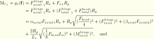
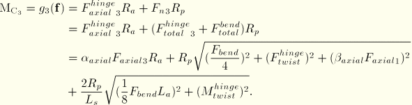
The moment magnitudes of the frictional tangential tractions are ![]() and
and ![]() .
.
| UJOINT | |
|---|---|
| Basic or assembled: | Assembled |
| Kinematic constraints: | JOIN + UNIVERSAL |
| Constraint force and moment output: | |
| Available components: | |
| Kinetic force and moment output: | |
| Orientation at a: | Required |
| Orientation at b: | Optional |
| Connector stops: | |
| Constitutive reference lengths and angles: | |
| Predefined friction parameters: | Required: |
| Contact moments for predefined friction: | |
Connection type UNIVERSAL provides a connection between two nodes where the rotations are fixed about one local direction and free about two others. Connection type UNIVERSAL provides the rotational part of a U-joint. Connection type UNIVERSAL cannot be used in two-dimensional or axisymmetric analysis.
A UNIVERSAL connection constrains the rotation about the shaft directions at two nodes. The shaft directions at nodes a and b are ![]() and
and ![]() , respectively. A UNIVERSAL connection requires that local direction
, respectively. A UNIVERSAL connection requires that local direction ![]() be perpendicular to
be perpendicular to ![]() . This single constraint is written
. This single constraint is written
![]()
The constraint moment imposed by the UNIVERSAL connection is
![]()
A UNIVERSAL connection allows two free rotational degrees of freedom between two nodes. The first and third Cardan angles that position local directions at node b relative to those at node a are
![]()
![]()
![]()
The kinetic moment in the UNIVERSAL connection is
![]()
When used by itself, there is no predefined Coulomb-like friction in the UNIVERSAL connection. However, when the UNIVERSAL connection is used in combination with the JOIN connection type, the predefined friction is the same as the UJOINT connection.
Connection type WELD provides a fully bonded connection between two nodes.
Connection type WELD imposes kinematic constraints and uses local orientation definitions equivalent to combining connection types JOIN and ALIGN.
| WELD | |
|---|---|
| Basic or assembled: | Assembled |
| Kinematic constraints: | JOIN + ALIGN |
| Constraint force and moment output: | |
| Available components: | None |
| Kinetic force and moment output: | None |
| Orientation at a: | Optional |
| Orientation at b: | Optional |
| Connector stops: | None |
| Constitutive reference lengths and angles: | None |
| Predefined friction parameters: | None |
| Contact force for predefined friction: | None |