Product: ABAQUS/Standard
Elbow elements:
are intended to provide accurate modeling of the nonlinear response of initially circular pipes and pipebends when distortion of the cross-section by ovalization and warping dominates the behavior;
appear as beams but are shells with quite complex deformation patterns allowed;
use plane stress theory to model the deformation through the pipe wall;
cannot provide nodal values of stress, strain, and other constitutive results; and
cannot be used to generate contour plots.
In the usual approach to linear analysis of elbows, the response prediction is based on semianalytical results, used as “flexibility factors” to correct results obtained with simple beam theory. Such factors do not apply in nonlinear cases, and the pipeline must be modeled as a shell to predict the response accurately (for example, see “Parametric study of a linear elastic pipeline under in-plane bending,” Section 1.1.3 of the ABAQUS Example Problems Manual). Although the elbow elements appear as beams, they are, in fact, shells, with quite complex deformation patterns allowed. In thin-walled elbows the interaction of elbows and adjacent straight segments is an important aspect of elbow modeling, as are the large rotations that readily occur in the cross-sectional deformation, even at small relative rotations of the pipe axis itself. All of these effects (including the stiffening effect of internal pressure) can be modeled with these elements.
Elbow elements are intended to provide accurate modeling of the nonlinear response of initially circular pipes and pipebends when distortion of the cross-section by ovalization and warping dominates the behavior. Such behavior arises in two circumstances: in pipebends, where the initial curvature of the pipe, together with the thinness of the wall of the pipe, causes ovalization to dominate the response, and in straight pipe sections, where excessive bending can lead to a buckling collapse of the thin-walled circular section (“Brazier buckling”).
Because the elbow elements use a full shell formulation around the circumference, the number of degrees of freedom per element is high. Elbow elements that use all Fourier modes (discussed below) to model ovalization and warping are considerably more expensive computationally than beam elements, but their cost is comparable to that of coarse shell models, which can be used to model the section.
If an analysis requires connecting pipe elements to a pipebend, it is easier to connect elbow elements to pipe elements than it is to connect shell elements to pipe elements.
Elbow elements use polynomial interpolation along their length (linear or quadratic depending on the element type), together with Fourier interpolation around the pipe to model the ovalization and warping of the section. Shell theory is then used to model the behavior.
Two types of elbow elements are provided.
Element types ELBOW31 and ELBOW32 are the most complete elbow elements. In these elements the ovalization of the pipe wall is made continuous from one element to the next, thus modeling such effects as the interaction between pipe bends (elbows) and adjacent straight segments of the pipeline.
ELBOW31 and ELBOW32 should not be used for the analysis of unconnected straight pipes unless the warping and ovalization are restrained at some point in the pipe.
Element types ELBOW31B and ELBOW31C use a simplified version of the formulation, in which ovalization only is considered (no warping) and axial gradients of the ovalization are neglected. These approximations are often satisfactory, and indeed they form the basis of the standard flexibility factor approach used in linear analysis of piping systems. They provide a considerably less expensive capability. ELBOW31C includes the further approximation that the odd numbered terms in the Fourier interpolation around the pipe, except the first term, are neglected. This formulation provides a slightly less expensive model for cases where the radius of the pipe is small compared to the radius of curvature of the pipe axis.
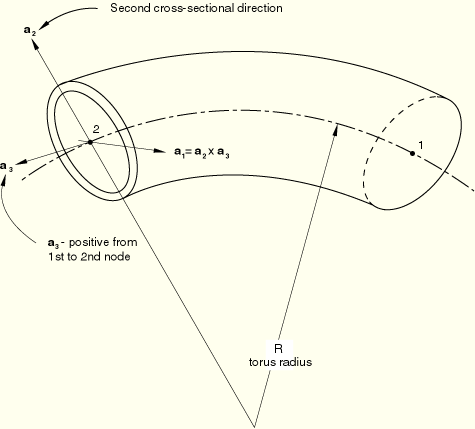
You use a beam section definition integrated during the analysis to define the section properties of elbow elements. Give the outside radius of the pipe, r; pipe wall thickness, t; and elbow torus radius, measured to the pipe axis, R. For a straight pipe, set R to zero.
You must associate these properties with a set of elbow elements.
| Input File Usage: | *BEAM SECTION, SECTION=ELBOW, ELSET=name r, t, R |
For all elbow elements the section must be oriented in space by specifying a point that, together with the nodes of the element, defines the plane of the ![]() -axis in Figure 23.5.1–1. For pipebends this point should be the point of intersection of the tangents to the adjacent straight pipe runs. When the elements are used to model straight pipes, the point can be any point off the pipe axis.
-axis in Figure 23.5.1–1. For pipebends this point should be the point of intersection of the tangents to the adjacent straight pipe runs. When the elements are used to model straight pipes, the point can be any point off the pipe axis.
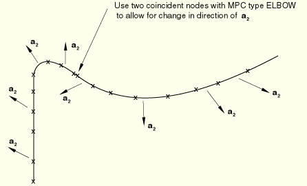
When ovalization modeling is extended onto straight runs adjacent to a pipebend by using ELBOW31 or ELBOW32 elements for the pipebend and for the straight pipe, you must ensure that the ![]() -axis is defined so that its orientation about the axis of the pipe is the same between the pipebend and each of the straight segments. When possible, the
-axis is defined so that its orientation about the axis of the pipe is the same between the pipebend and each of the straight segments. When possible, the ![]() -axis should also be the same between adjacent pipebends. In some cases, such as adjacent pipebends in different planes, the
-axis should also be the same between adjacent pipebends. In some cases, such as adjacent pipebends in different planes, the ![]() -axes are necessarily discontinuous. In such cases separate nodes must be introduced at the point where the
-axes are necessarily discontinuous. In such cases separate nodes must be introduced at the point where the ![]() -axis changes orientation, and MPC type ELBOW must be invoked to impose the appropriate constraints to ensure continuity of displacements. See Figure 23.5.1–2.
-axis changes orientation, and MPC type ELBOW must be invoked to impose the appropriate constraints to ensure continuity of displacements. See Figure 23.5.1–2.
| Input File Usage: | *BEAM SECTION, SECTION=ELBOW first data line coordinates of orientation point |
You can specify the number of integration points and Fourier modes for an elbow section. Experience suggests that for relatively thick-walled cases 4 Fourier modes with 12 integration points around the pipe are sufficient. For thin-walled elbows 6 Fourier modes and 18 integration points around the pipe are needed. As a general rule, the number of integration points around the pipe should not be less than three times the number of Fourier modes used; otherwise, singularities may arise in the stiffness matrix. When used with zero Fourier modes, the elements become simple pipe elements with hoop strain and stress included: when Poisson's ratio is set to zero, they show similar behavior to the PIPE elements in ABAQUS (see “Choosing a beam element,” Section 23.3.3).
| Input File Usage: | *BEAM SECTION, SECTION=ELBOW first data line second data line number of int. pts. through thickness, number of int. pts. around pipe, number of Fourier modes |
You must associate a material definition with each elbow section definition.
| Input File Usage: | *BEAM SECTION, SECTION=ELBOW, MATERIAL=name |
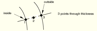
Temperature and field variables can be specified by defining the values at specific points through the section or by defining the value at the middle of the pipe wall and specifying the gradient through the pipe thickness.
You can define temperatures and field variables by giving the values at each of the three points shown below.
| Input File Usage: | *BEAM SECTION, SECTION=ELBOW, TEMPERATURE=VALUES |
Alternatively, you can define temperatures and field variables by giving the value on the middle surface of the pipe wall and the gradient of temperature with respect to position through the pipe wall thickness, positive when the outside surface is hotter than the inside surface.
| Input File Usage: | *BEAM SECTION, SECTION=ELBOW, TEMPERATURE=GRADIENTS |
When elbow elements are subjected to pipe pressure loads (load types PI, PE, HPI, or HPE) in large-displacement analysis (“General and linear perturbation procedures,” Section 6.1.2), the most significant contributions to the load stiffness are taken into account.
Kinematic boundary conditions on the standard degrees of freedom at the nodes of elbow elements (that is, degrees of freedom 1–6) should be treated in the usual way.
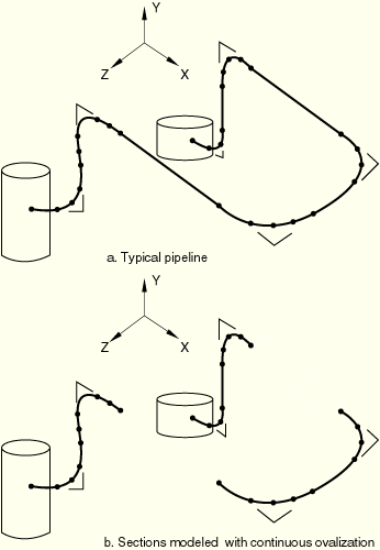
In addition, the elements have ovalization and warping terms stored internally. For ELBOW31B and ELBOW31C elements this requires no additional consideration. For ELBOW31 or ELBOW32 elements you may often need to provide kinematic boundary conditions on these additional degrees of freedom. For example, it is common to model a pipeline with ovalization and warping allowed in the elbows and adjacent straight pipe segments but no ovalization in the middle segments of long, straight pipe runs (see Figure 23.5.1–3).
(The latter is usually accomplished by specifying ELBOW31 elements with zero modes or PIPE31 elements so that the usual bending terms and the uniform radial expansion term, associated with pressure in the pipe, are included; if internal pressure is not important, a simple beam element, B31, can be used instead.) Where the segments with ovalization and warping end, the warping must be restrained; and if a stiff flange or vessel exists at that point, the ovalization should also be restrained. To do so, specify NOWARP and/or NOOVAL or NODEFORM boundary conditions for that node (“Boundary conditions,” Section 27.3.1).NOWARP means that no warping is allowed at the node, but ovalization and uniform radial expansion are allowed; NOOVAL means that there can be no ovalization at the node, but warping and uniform radial expansion are allowed; NODEFORM means that there can be no cross-section deformation at all—no warping, ovalization, or uniform radial expansion.
Typically, NOWARP will be specified at the end of a pipebend segment modeled with ELBOW31 adjacent to a straight pipe run, while NOWARP and NOOVAL would be specified at a stiff flange or vessel attachment point. NODEFORM restrains all cross-sectional deformation, including the uniform radial expansion term: this will result in large stresses if thermal expansion occurs. NODEFORM should be used, for example, at a built-in end.
The current release of ABAQUS/Standard does not provide a direct way of visualizing the cross-section ovalization. However, the utility routine felbow.f (“Creation of a data file to facilitate the postprocessing of elbow element results: FELBOW,” Section 12.1.6 of the ABAQUS Example Problems Manual) creates a data file that can be used in ABAQUS/CAE to plot the current coordinates of the integration points around the circumference of the elbow section of interest. The routine uses output variable COORD (“ABAQUS/Standard output variable identifiers,” Section 4.2.1) to obtain the current coordinates of the integration points. These values are available only if geometric nonlinearity is considered in the step. You will have to ensure that the variable COORD is written to the results (.fil) file for this purpose.
The routine is suitable for elbow elements oriented arbitrarily in space: the integration points of the elbow section are projected appropriately to a coordinate system suitable for plotting the cross-section. The input data for plotting are written to a file that can be read into ABAQUS/CAE. An X–Y plot of the elbow element's deformed cross-section can be displayed using the XY Data Manager in the Visualization module.
In addition to facilitating the visualization of the cross-section ovalization, the program also allows you to create data files to plot the variation of a variable along a line of elbow elements and around the circumference of a given elbow element.
Similar C++ and Python utility routines, felbow.C (“A C++ version of FELBOW,” Section 9.15.6 of the ABAQUS Scripting User's Manual) and felbow.py (“An ABAQUS Scripting Interface version of FELBOW,” Section 8.10.12 of the ABAQUS Scripting User's Manual), are provided to process the pertinent elbow element results output written to the output database (.odb) file. When these programs are executed, they write data to an ASCII format file and/or an output database file that can be used in ABAQUS/CAE to plot the current coordinates of the integration points around the circumference of the elbow section. Both these routines can also be used to visualize the variation of an output variable around the circumference of the elbow section.