Products: ABAQUS/Standard ABAQUS/CAE
ALE adaptive meshing consists of two fundamental tasks:
creating a new mesh through a process called sweeping, and
remapping solution variables from the old mesh to the new mesh with a process called advection.
Adaptive mesh smoothing is defined as part of a step definition. The adaptive meshing in ABAQUS/Standard uses an operator split method wherein each analysis increment consists of a Lagrangian phase followed by an Eulerian phase. The Lagrangian phase is the typical ABAQUS/Standard solution increment where neither mesh sweeps nor advection occur. Once the equilibrium equations have converged, mesh smoothing is applied. Following the adjustment of nodes through the mesh sweeping process, material point quantities are advected in an Eulerian phase to account for the revised meshing of the model in its current configuration. This operator split method is chosen to avoid unsymmetric Jacobian terms that would result when the advection and material straining occur simultaneously. Advection is not required for, and is not applied to, acoustic elements.
Adaptive mesh smoothing is performed after the structural equilibrium equations have converged. The mesh smoothing equations are solved explicitly by sweeping iteratively over the adaptive mesh domain. During each mesh sweep, nodes in the domain are relocated—based on the positions of neighboring nodes obtained during the previous mesh sweep—to reduce element distortion. The new position, ![]() , of a node is obtained as
, of a node is obtained as
![]()
Original configuration projection is the default in ABAQUS/Standard and determines the weight function from a least squares minimization procedure that minimizes node displacement in a projection of the mesh back to the original configuration. This method of smoothing affects only deformations of the mesh and not the original mesh.
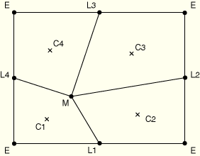
Volume smoothing determines the weight function by computing a volume-weighted average of the element centers in the elements surrounding the node. In Figure 12.2.7–1 the new position of node M is determined by a volume-weighted average of the positions of the element centers, C, of the four surrounding elements. The volume weighting will tend to push the node away from element center C1 and toward element center C3, thus reducing element distortion.
Volume smoothing is supported in structured domains, where every node is surrounded by four elements in two dimensions or eight elements in three dimensions.
The default smoothing method in ABAQUS/Standard is original configuration projection. To choose an alternate smoothing method or to combine the smoothing methods, you specify the weighting factor for each method. When more than one smoothing method is used, a node is relocated by computing a weighted average of the locations predicted by each chosen method. All weights must be zero or positive, and their sum must be nonzero. The weights are significant only in a relative sense; their values are normalized so that their sum is 1.0.
| Input File Usage: | *ADAPTIVE MESH CONTROLS, NAME=name original configuration projection weight, volume smoothing weight |
For example, the following option could be used to define an equal blend of original configuration projection and volume smoothing: *ADAPTIVE MESH CONTROLS, NAME=name 0.5, 0.5 |
| ABAQUS/CAE Usage: | Step module: Other |
The conventional forms of the basic smoothing methods may not perform well in highly distorted domains. You can use geometrically enhanced forms of the basic smoothing algorithms as a technique to mitigate distortion. These forms are heuristic and based on nodal locations only. Due to their heuristic nature, geometric enhancements may not always improve the mesh smoothing.
| Input File Usage: | Use the following option to apply geometric enhancements to the smoothing algorithm: |
*ADAPTIVE MESH CONTROLS, NAME=name, GEOMETRIC ENHANCEMENT=YES |
| ABAQUS/CAE Usage: | Step module: Other |
The mesh smoothing process begins with the mesh in its current displaced equilibrium configuration. Nodes that have no displacement degrees of freedom, such as those connected to acoustic elements, are maintained at their most recent configuration. Mesh smoothing is then driven by distortions in the current configuration and by boundary constraints. These boundary constraints can be described directly through adaptive mesh constraints. In the case of structural-acoustic boundaries the structural mesh boundary provides a constraint that controls the smoothing of adjacent acoustic element regions.
When these boundary constraints are much larger than the characteristic element length in the adaptive mesh domain, significant geometric changes, such as the development of corners, can occur. To prevent such changes, the constraints are applied gradually over a series of “sub-increments” onto the domain boundary. The number of sub-increments used is determined on the basis of the magnitude of the maximum surface displacement and the characteristic element dimension.
The remaining nodes (nodes not driven by constraints) are identified as interior nodes, free surface nodes, edge nodes, or corner nodes. These nodes are treated as described in “Defining ALE adaptive mesh domains in ABAQUS/Standard,” Section 12.2.6.
At the end of mesh sweeping the new geometry is checked to ensure that elements did not become severely distorted during mesh smoothing. ABAQUS/Standard responds to severe distortion in different ways, depending on the elements and procedures used. When adaptive meshing is used with acoustic elements, the current analysis increment is repeated with a reduced time increment, followed by another adaptive mesh smoothing attempt. When adaptive meshing is used with other elements, severe distortion results in abandonment of mesh smoothing for that increment. In cases where adaptive mesh constraints are also defined, ABAQUS/Standard aborts since the constraints cannot be satisfied.
In most cases the frequency of adaptive meshing is the parameter that most affects the mesh quality. By default, mesh smoothing will be performed after each converged structural analysis increment. You can change the frequency of adaptive meshing, except when adaptive mesh constraints are defined.
| Input File Usage: | *ADAPTIVE MESH, FREQUENCY=number of increments |
| ABAQUS/CAE Usage: | Step module: Other |
The adaptive mesh smoothing equations are solved explicitly by sweeping iteratively over the adaptive mesh domain. During each mesh sweep, nodes in the domain are relocated based on the current positions of neighboring nodes to reduce element distortion.
Mesh smoothing is performed following the end of a converged increment. You can control the intensity of the mesh smoothing by defining the number of mesh sweeps required. When the displacements are large, more iterations are usually required. When used in acoustic analyses, more iterations are usually required when the volume of the elements in the acoustic domain decreases compared to the case when the volume increases during structural loading.
You can specify the number of mesh sweeps to be performed in each adaptive mesh increment. The default number of mesh sweeps is one.
By applying the mesh sweeping algorithm repeatedly, the mesh will converge; in other words, nodal positions are obtained that do not change with further mesh sweeping. However, it is usually not necessary to apply mesh smoothing until a converged mesh is obtained; the main objective is to reduce element distortion.
| Input File Usage: | *ADAPTIVE MESH, MESH SWEEPS=number of sweeps |
| ABAQUS/CAE Usage: | Step module: Other |
ABAQUS/Standard applies an explicit method, based on the Lax-Wendroff method, to integrate the advection equation. The key principle of the Lax-Wendroff method is replacement of the time derivatives of the material point quantities with the spatial derivatives using the classical relationship between the material time derivative, the referential derivative, and the spatial derivative. The update scheme is second-order accurate and provides some upwinding. Nodal quantities are advected by first converting them to the material point quantities.
Advection of the material quantities will generally result in loss of equilibrium, for two main reasons. The first reason is the errors in the advection process itself. To minimize the errors in advection, ABAQUS/Standard imposes restrictions on the magnitude of the advection velocity by requiring that the Courant number for every element in the adaptive domain be less than one. In cases where the Courant number is greater than one you will be informed and ABAQUS/Standard will generate multiple advection passes per increment. The second reason for the loss of equilibrium is changes in the representation of the underlying material quantities by the changed mesh. For example, consider a region of the structure having some stress gradients spanned initially by two elements. After mesh smoothing, the same region might have more than two elements. This will lead to slightly different volume integration while computing the internal force even when there are no errors in advection.
These sources of error in equilibrium are significant only when the mesh is too coarse to provide a good solution and mesh smoothing is carried out with such small frequency that the mesh motion is larger than the average element size. In practical applications these errors are typically insignificant, the resulting loss of equilibrium is generally small, and the residuals generated by the loss of the equilibrium fall within the limits of the ABAQUS/Standard convergence criterion. Any loss of equilibrium is not propagated since equilibrium will again be satisfied at the end of the Lagrangian phase of the next increment.
To ensure that the results are output only for the configuration that satisfies equilibrium, ABAQUS/Standard always outputs the results at the end of the Lagrangian phase. The Eulerian phase that follows the Lagrangian phase will leave the structure out of equilibrium for the next increment. This sequence has a consequence that after the last Eulerian phase is carried out at the end of the step, equilibrium will not be satisfied exactly at the beginning of the next step and the solution at the end of the step will differ slightly from the solution at the zero increment of the following step. Equilibrium can again be established by following the step that had adaptive meshing by a step that removes all the adaptive mesh domains and allows the structure to equilibrate. A one-increment step will usually suffice. This is particularly important when the following step is a perturbation procedure that uses the solution from the previous step as the base state.
Frequency steps that follow adaptive mesh steps will also be impacted, because element mass is not advected during mesh smoothing. This impact on the element mass can be significant, depending on the extent of adaptive mesh motion and change in element size due to mesh smoothing. ABAQUS will provide a warning message in cases where adaptive meshing precedes a frequency step; you should evaluate the impact of your updated mesh configuration when interpreting results from a frequency step in these cases.
In adaptive meshing the integration point of an element will generally not refer to the same material point throughout the analysis. Contour plots of material variables will show correct spatial distribution, but history plots are not meaningful. The displacement of the nodes contains the material displacement as well as the displacement due to mesh motion. You can obtain measures of the volume lost due to adaptive mesh constraints with the partial model variable VOLC, which is useful when using adaptive mesh constraints to model ablation.
A summary of the adaptive meshing in each adaptive mesh domain is written to the message (.msg) file. This summary includes the total number of load increments over which the structural displacement is transferred to the fluid, the total number of mesh sweeps performed, the magnitude of the maximum displacement increment, and the node and degree of freedom at which the maximum displacement increment is measured. Warning messages are issued when geometric features change during mesh smoothing.
More detailed diagnostic output for adaptive mesh smoothing can be requested; see “The ABAQUS/Standard message file” in “Output,” Section 4.1.1. This output provides the magnitude of the maximum displacement and the node and degree of freedom where the maximum displacement increment occurs during each mesh sweep. In addition, the nodes experiencing changes in geometric features are listed.
Lax, P. D., and B. Wendroff, “Systems of Conservations Laws,” Communications on Pure and Applied Mathematics, vol. 13, pp. 217–237, 1960.
Lax, P. D., and B. Wendroff, “Difference Schemes for Hyperbolic Equations with High-Order Accuracy,” Communications on Pure and Applied Mathematics, vol. 17 381, 1964.