Products: ABAQUS/Standard ABAQUS/CAE
A mode-based steady-state dynamic analysis:
is used to calculate the steady-state dynamic linearized response of a system to harmonic excitation;
is a linear perturbation procedure;
calculates the response based on the system's eigenfrequencies and modes;
requires that an eigenfrequency extraction procedure be performed prior to the steady-state dynamic analysis;
is an alternative to direct-solution steady-state dynamic analysis, in which the system's response is calculated in terms of the physical degrees of freedom of the model;
is computationally cheaper than direct-solution or subspace-based steady-state dynamics;
is less accurate than direct-solution or subspace-based steady-state analysis, in particular if significant material damping is present; and
is able to bias the excitation frequencies toward the values that generate a response peak.
Steady-state dynamic analysis provides the steady-state amplitude and phase of the response of a system due to harmonic excitation at a given frequency. Usually such analysis is done as a frequency sweep by applying the loading at a series of different frequencies and recording the response; in ABAQUS/Standard the steady-state dynamic analysis procedure is used to conduct the frequency sweep.
In a mode-based steady-state dynamic analysis the response is based on modal superposition techniques; the modes of the system must first be extracted using the eigenfrequency extraction procedure. The modes will include eigenmodes and, if activated in the eigenfrequency extraction step, residual modes. The number of modes extracted must be sufficient to model the dynamic response of the system adequately, which is a matter of judgment on your part.
When defining a mode-based steady-state dynamic step, you specify the frequency ranges of interest and the number of frequencies at which results are required in each range (including the bounding frequencies of the range). In addition, you can specify the type of frequency spacing (linear or logarithmic) to be used, as described below (“Selecting the frequency spacing”). Logarithmic frequency spacing is the default. Frequencies are given in cycles/time.
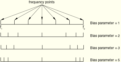
These frequency points for which results are required can be spaced equally along the frequency axis (on a linear or a logarithmic scale), or they can be biased toward the ends of the user-defined frequency range by introducing a bias parameter (see “The bias parameter,” below).
While the response in this procedure is for linear vibrations, the prior response can be nonlinear. Initial stress effects (stress stiffening) will be included in the steady-state dynamics response if nonlinear geometric effects (“General and linear perturbation procedures,” Section 6.1.2) were included in any general analysis step prior to the eigenfrequency extraction step preceding the steady-state dynamic procedure.
| Input File Usage: | *STEADY STATE DYNAMICS |
The DIRECT and SUBSPACE PROJECTION parameters must be omitted from the *STEADY STATE DYNAMICS option to conduct a mode-based steady-state dynamic analysis. |
| ABAQUS/CAE Usage: | Step module: Create Step: Linear perturbation: Steady-state dynamics, Modal |
Two types of frequency intervals are permitted for output from a mode-based steady-state dynamic step.
By default, the eigenfrequency type of frequency interval is used; in this case the following intervals exist in each frequency range:
First interval: extends from the lower limit of the frequency range given to the first eigenfrequency in the range.
Intermediate intervals: extend from eigenfrequency to eigenfrequency.
Last interval: extends from the highest eigenfrequency in the range to the upper limit of the frequency range.
| Input File Usage: | *STEADY STATE DYNAMICS, INTERVAL=EIGENFREQUENCY |
| ABAQUS/CAE Usage: | Step module: Create Step: Linear perturbation: Steady-state dynamics, Modal: Use eigenfrequencies to subdivide each frequency range |
If the alternative range type of frequency interval is chosen, there is only one interval in the specified frequency range spanning from the lower to the upper limit of the range. This interval is divided using the user-defined number of points and the optional bias function, which can be used to space the sampling frequency points closer to the range limits. For the range type of frequency interval, the peak responses around the system's eigenfrequencies may be missed since the sampling frequencies at which output will be reported will not be biased toward the eigenfrequencies.
| Input File Usage: | *STEADY STATE DYNAMICS, INTERVAL=RANGE |
| ABAQUS/CAE Usage: | Step module: Create Step: Linear perturbation: Steady-state dynamics, Modal: toggle off Use eigenfrequencies to subdivide each frequency range |
Two types of frequency spacing are permitted for a mode-based steady-state dynamic step. For the logarithmic frequency spacing (the default), the specified frequency ranges of interest are divided using a logarithmic scale. Alternatively, a linear frequency spacing can be used if a linear scale is desired.
| Input File Usage: | Use either of the following options: |
*STEADY STATE DYNAMICS, FREQUENCY SCALE=LOGARITHMIC *STEADY STATE DYNAMICS, FREQUENCY SCALE=LINEAR |
| ABAQUS/CAE Usage: | Step module: Create Step: Linear perturbation: Steady-state dynamics, Modal: Scale: Logarithmic or Linear |
You can request multiple frequency ranges or multiple single frequency points for a mode-based steady-state dynamic step.
| Input File Usage: | *STEADY STATE DYNAMICS lower_frequency1, upper_frequency1, number_of_points1, bias_parameter1 lower_frequency2, upper_frequency2, number_of_points2, bias_parameter2 ... single_frequency1 single_frequency2 ... |
Repeat the data lines as often as necessary. When both frequency ranges and additional single frequency points are requested, the frequency ranges must be specified first. |
| ABAQUS/CAE Usage: | Step module: Create Step: Linear perturbation: Steady-state dynamics, Modal: Data: enter data in table, and add rows as necessary |
The bias parameter can be used to provide closer spacing of the results points either toward the middle or toward the ends of each frequency interval. Figure 6.3.8–2 shows a few examples of the effect of the bias parameter on the frequency spacing.
The bias formula used to calculate the frequency at which results are presented is as follows:
![]()
y
![]() ;
;
n
is the number of frequency points at which results are to be given within a frequency interval (discussed above);
k
is one such frequency point (![]() );
);
![]()
is the lower limit of the frequency interval;
![]()
is the upper limit of the frequency interval;
![]()
is the frequency at which the kth results are given;
p
is the bias parameter value; and
![]()
is the frequency or the logarithm of the frequency, depending on the value used for the frequency scale parameter.
You can select the modes to be used in modal superposition and specify damping values for all selected modes.
You can select modes by specifying the mode numbers individually, by requesting that ABAQUS/Standard generate the mode numbers automatically, or by requesting the modes that belong to specified frequency ranges. If you do not select the modes, all modes extracted in the prior eigenfrequency extraction step, including residual modes if they were activated, are used in the modal superposition.
| Input File Usage: | Use one of the following options to select the modes by specifying mode numbers: |
*SELECT EIGENMODES, DEFINITION=MODE NUMBERS
*SELECT EIGENMODES, GENERATE, DEFINITION=MODE NUMBERS
Use the following option to select the modes by specifying a frequency range: *SELECT EIGENMODES, DEFINITION=FREQUENCY RANGE |
| ABAQUS/CAE Usage: | You cannot select the modes in ABAQUS/CAE; all modes extracted are used in the modal superposition. |
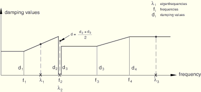
Damping is almost always specified for a steady-state analysis (see “Material damping,” Section 20.1.1). If damping is absent, the response of a structure will be unbounded if the forcing frequency is equal to an eigenfrequency of the structure. To get quantitatively accurate results, especially near natural frequencies, accurate specification of damping properties is essential. The various damping options available are discussed in “Material damping,” Section 20.1.1. You can define a damping coefficient for all or some of the modes used in the response calculation. The damping coefficient can be given for a specified mode number or for a specified frequency range. When damping is defined by specifying a frequency range, the damping coefficient for a mode is interpolated linearly between the specified frequencies. The frequency range can be discontinuous; the average damping value will be applied for an eigenfrequency at a discontinuity. The damping coefficients are assumed to be constant outside the range of specified frequencies.
| Input File Usage: | Use the following option to define damping by specifying mode numbers: |
*MODAL DAMPING, DEFINITION=MODE NUMBERS Use the following option to define damping by specifying a frequency range: *MODAL DAMPING, DEFINITION=FREQUENCY RANGE |
| ABAQUS/CAE Usage: | Use the following input to define damping by specifying mode numbers: |
Step module: Create Step: Linear perturbation: Steady-state dynamics, Modal: Damping Defining damping by specifying frequency ranges is not supported in ABAQUS/CAE. |
Figure 6.3.8–3 illustrates how the damping coefficients at different eigenfrequencies are determined for the following input:
*MODAL DAMPING, DEFINITION=FREQUENCY RANGE


The following rules apply for selecting modes and specifying modal damping coefficients:
No modal damping is included by default.
Mode selection and modal damping must be specified in the same way, using either mode numbers or a frequency range.
If you do not select any modes, all modes extracted in the prior frequency analysis, including residual modes if they were activated, will be used in the superposition.
If you do not specify damping coefficients for modes that you have selected, zero damping values will be used for these modes.
Damping is applied only to the modes that are selected.
Damping coefficients for selected modes that are beyond the specified frequency range are constant and equal to the damping coefficient specified for the first or the last frequency (depending which one is closer). This is consistent with the way ABAQUS interprets amplitude definitions.
The base state is the current state of the model at the end of the last general analysis step prior to the steady-state dynamic step. If the first step of an analysis is a perturbation step, the base state is determined from the initial conditions (“Initial conditions,” Section 27.2.1). Initial condition definitions that directly define solution variables, such as velocity, cannot be used in a steady-state dynamic analysis.
In a mode-based steady-state dynamic analysis both the real and imaginary parts of any degree of freedom are either restrained or unrestrained; it is physically impossible to have one part restrained and the other part unrestrained. ABAQUS/Standard will automatically restrain both the real and imaginary parts of a degree of freedom even if only one part is restrained.
It is not possible to prescribe nonzero displacements and rotations directly as boundary conditions (“Boundary conditions,” Section 27.3.1) in mode-based dynamic response procedures. Therefore, in a mode-based steady-state dynamic analysis, the motion of nodes can be specified only as base motion; nonzero displacement or acceleration history definitions given as boundary conditions are ignored, and any changes in the support conditions from the eigenfrequency extraction step are flagged as errors. The method for prescribing base motion in modal superposition procedures is described in “Transient modal dynamic analysis,” Section 6.3.7.
An amplitude definition can be used to specify the amplitude of a base motion as a function of frequency (“Amplitude curves,” Section 27.1.2).
| Input File Usage: | Use both of the following options: |
*AMPLITUDE, NAME=name *BASE MOTION, LOAD CASE=n, AMPLITUDE=name |
| ABAQUS/CAE Usage: | Base motions are not supported in ABAQUS/CAE. |
The following loads can be prescribed in a mode-based steady-state dynamic analysis, as described in “Concentrated loads,” Section 27.4.2:
Concentrated nodal forces can be applied to the displacement degrees of freedom (1–6).
Distributed pressure forces or body forces can be applied; the distributed load types available with particular elements are described in Part VI, “Elements.”
Fluid flux loading cannot be used in a steady-state dynamic analysis.
| ABAQUS/CAE Usage: | Load module: load editor: real (in-phase) part + imaginary (out-of-phase) part i |
An amplitude definition can be used to specify the amplitude of a load as a function of frequency (“Amplitude curves,” Section 27.1.2).
| Input File Usage: | Use both of the following options: |
*AMPLITUDE, NAME=name *CLOAD or *DLOAD, LOAD CASE=n, AMPLITUDE=name |
| ABAQUS/CAE Usage: | Load or Interaction module: Create Amplitude: Name: name |
Load module: load editor: real (in-phase) part + imaginary (out-of-phase) part i: Amplitude: name |
Predefined temperature fields are not allowed in mode-based steady-state dynamic analysis. Other predefined fields are ignored.
As in any dynamic analysis procedure, mass or density (“Density,” Section 16.2.1) must be assigned to some regions of any separate parts of the model where dynamic response is required. The following material properties are not active during mode-based steady-state dynamic analyses: plasticity and other inelastic effects, viscoelastic effects, thermal properties, mass diffusion properties, electrical properties (except for the electrical potential, ![]() , in piezoelectric analysis), and pore fluid flow properties—see “General and linear perturbation procedures,” Section 6.1.2.
, in piezoelectric analysis), and pore fluid flow properties—see “General and linear perturbation procedures,” Section 6.1.2.
Any of the following elements available in ABAQUS/Standard can be used in a steady-state dynamics procedure:
stress/displacement elements (other than generalized axisymmetric elements with twist);
acoustic elements;
piezoelectric elements; or
hydrostatic fluid elements.
In mode-based steady-state dynamic analysis the value of an output variable such as strain (E) or stress (S) is a complex number with real and imaginary components. In the case of data file output the first printed line gives the real components while the second lists the imaginary components. Results and data file output variables are also provided to obtain the magnitude and phase of many variables (see “ABAQUS/Standard output variable identifiers,” Section 4.2.1). In the case of data file output the first printed line gives the magnitudes while the second lists the phase angle.
The following variables are provided specifically for steady-state dynamic analysis:
PHS | Magnitude and phase angle of all stress components. |
PHE | Magnitude and phase angle of all strain components. |
PHEPG | Magnitude and phase angles of the electrical potential gradient vector. |
PHEFL | Magnitude and phase angles of the electrical flux vector. |
PHMFL | Magnitude and phase angle of the mass flow rate in fluid link elements. |
PHMFT | Magnitude and phase angle of the total mass flow in fluid link elements. |
PHCTF | Magnitude and phase angle of connector total forces. |
PHCEF | Magnitude and phase angle of connector elastic forces. |
PHCVF | Magnitude and phase angle of connector viscous forces. |
PHCRF | Magnitude and phase angle of connector reaction forces. |
PHCSF | Magnitude and phase angle of connector friction forces. |
PHCU | Magnitude and phase angle of connector relative displacements. |
PHCCU | Magnitude and phase angle of connector constitutive displacements. |
PU | Magnitude and phase angle of all displacement/rotation components at a node. |
PPOR | Magnitude and phase angle of the fluid or acoustic pressure at a node. |
PHPOT | Magnitude and phase angle of the electrical potential at a node. |
PRF | Magnitude and phase angle of all reaction forces/moments at a node. |
PHCHG | Magnitude and phase angle of the reactive charge at a node. |
Element energy densities (such as the elastic strain energy density, SENER), whole element energies (such as the total kinetic energy of an element, ELKE), and NFORC (internal forces at the nodes of the elements) are not available for output in a mode-based steady-state dynamic analysis.
The standard output variables U, V, A, and the variable PU listed above correspond to motions relative to the motion of the primary base in a mode-based analysis. Total values, which include the motion of the primary base, are also available:
TU | Magnitude of all components of total displacement/rotation at a node. |
TV | Magnitude of all components of total velocity at a node. |
TA | Magnitude of all components of total acceleration at a node. |
PTU | Magnitude and phase angle of all total displacement/rotation components at a node. |
The following modal variables are also available for mode-based steady-state dynamic analysis and can be output to the data, results, and/or output database files (see “Output to the data and results files,” Section 4.1.2, and “Output to the output database,” Section 4.1.3):
GU | Generalized displacements for all modes. |
GV | Generalized velocities for all modes. |
GA | Generalized accelerations for all modes. |
GPU | Phase angle of generalized displacements for all modes. |
GPV | Phase angle of generalized velocities for all modes. |
GPA | Phase angle of generalized acceleration for all modes. |
SNE | Elastic strain energy for the entire model per mode. |
KE | Kinetic energy for the entire model per mode. |
T | External work for the entire model per mode. |
BM | Base motion. |
Whole model variables such as ALLIE (total strain energy) are available for mode-based steady-state dynamics as output to the data, results, and/or output database files (see “Output to the data and results files,” Section 4.1.2).
*HEADING
…
*AMPLITUDE, NAME=loadamp
Data lines to define an amplitude curve as a function of frequency (cycles/time)
*AMPLITUDE, NAME=base
Data lines to define an amplitude curve to be used to prescribe base motion
**
*STEP, NLGEOM
Include the NLGEOM parameter so that stress stiffening effects will
be included in the steady-state dynamics step
*STATIC
**Any general analysis procedure can be used to preload the structure
…
*CLOAD and/or *DLOAD
Data lines to prescribe preloads
*TEMPERATURE and/or *FIELD
Data lines to define values of predefined fields for preloading the structure
*BOUNDARY
Data lines to specify boundary conditions to preload the structure
*END STEP
**
*STEP
*FREQUENCY
Data line to control eigenvalue extraction
*BOUNDARY
Data lines to assign degrees of freedom to the primary base
*BOUNDARY, BASE NAME=base2
Data lines to assign degrees of freedom to a secondary base
*END STEP
**
*STEP
*STEADY STATE DYNAMICS
Data lines to specify frequency ranges and bias parameters
*SELECT EIGENMODES
Data lines to define the applicable mode ranges
*MODAL DAMPING
Data lines to define the modal damping factors
*BASE MOTION, DOF=dof, AMPLITUDE=base
*BASE MOTION, DOF=dof, AMPLITUDE=base, BASE NAME=base2
*CLOAD and/or *DLOAD, AMPLITUDE=loadamp
Data lines to specify sinusoidally varying, frequency-dependent loads
…
*END STEP