2.16.2 Stress intensity factor extraction

The stress intensity factors  ,
,  , and
, and  play an important role in linear elastic fracture mechanics. They characterize the influence of load or deformation on the magnitude of the crack-tip stress and strain fields and measure the propensity for crack propagation or the crack driving forces. Furthermore, the stress intensity can be related to the energy release rate (the J-integral) for a linear elastic material through
where
and

is called the pre-logarithmic energy factor matrix (
Shih and Asaro, 1988;
Barnett and Asaro, 1972;
Gao, Abbudi, and Barnett, 1991;
Suo, 1990). For homogeneous, isotropic materials
is diagonal and the above equation simplifies to
where

for plane stress and
for plane strain, axisymmetry, and three dimensions. For an interfacial crack between two dissimilar isotropic materials with Young's moduli

and

, Poisson's ratios

and

, and shear moduli
and
,
where
and

for plane strain, axisymmetry, and three dimensions; and
for plane stress. Unlike their analogues in a homogeneous material,
and
are no longer the pure Mode I and Mode II stress intensity factors for an interfacial crack. They are simply the real and imaginary parts of a complex stress intensity factor, whose physical meaning can be understood from the interface traction expressions:
where
r and

are polar coordinates centered at the crack tip. The bimaterial constant

is defined as
In this section we describe an interaction integral method (Shih and Asaro, 1988) to extract the individual stress intensity factors for a crack under mixed-mode loading. The method is applicable to cracks in isotropic and anisotropic linear materials.
Interaction integral method
In general, the J-integral for a given problem can be written as
where

correspond to

when indicating the components of
B. We define the
J-integral for an auxiliary, pure Mode I, crack-tip field with stress intensity factor

as
Superimposing the auxiliary field onto the actual field yields
Since the terms not involving or  in
in  and J are equal, the interaction integral can be defined as
If the calculations are repeated for Mode  and Mode
  , a linear system of equations results:
If the

are assigned unit values, the solution of the above equations leads to
where
The calculation of this integral is discussed next.
Based on the definition of the J-integral, the interaction integrals  can be expressed as
with

given as
The subscript

represents three auxiliary pure Mode I, Mode II, and Mode III crack-tip fields for
, respectively.

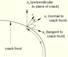
is a contour that lies in the normal plane at position
s along the crack front, beginning on the bottom crack surface and ending on the top surface (see
Figure 2.16.2–1). The limit

indicates that
shrinks onto the crack tip.
Following the domain integral procedure used in ABAQUS/Standard for calculating the J-integral, we define an interaction integral for a virtual crack advance  :
:
where
L denotes the crack front under consideration;

is a surface element on a vanishingly small tubular surface enclosing the crack tip (i.e.,

);

is the outward normal to
; and

is the local direction of virtual crack propagation. The integral

can be calculated by the same domain integral method as that used for calculating the
J-integral.
To obtain at each node set P along the crack front line,  is discretized with the same interpolation functions as those used in the finite elements along the crack front:
where

at the node set
P and all other

are zero. The result is substituted into the expression for

. Finally, the interaction integral value at each node set
P along the crack front can be calculated as