Under certain loading conditions linear reduced-integration elements can experience a pattern of nonphysical deformation called hourglassing. Consider a single first-order, reduced-integration element modeling a small piece of material subjected to pure bending, as shown in Figure 4–8. Dotted visualization lines are shown passing through the single integration point in the element.
Figure 4–8 Deformation of a first-order element with reduced integration subjected to a bending moment.
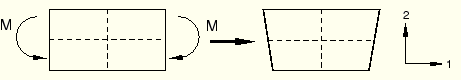
As the element deforms, neither of the dotted visualization lines changes in length, and the angle between them also does not change. Therefore, all components of stress and strain at the element's single integration point are zero. This deformation mode is, therefore, a zero-energy mode because no strain energy is generated by distorting the element in this manner. The element is unable to resist this type of deformation since it has no stiffness in this mode. In coarse meshes this zero-energy mode can propagate through the mesh, producing incorrect results.
ABAQUS/Explicit has first-order, reduced-integration quadrilateral and hexahedral elements that have hourglass modes. Hourglassing can, therefore, sometimes propagate through a mesh. ABAQUS/Explicit includes sophisticated controls to prevent hourglassing from being a problem in most real analyses. However, the hourglass controls work by applying corrective forces and may take a few increments to control hourglassing. In some severe cases hourglassing can propagate through the mesh before the hourglass controls can correct the problem. This example illustrates such a modeling situation.
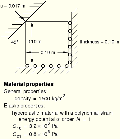
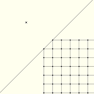
In this example you will consider a thick rubber block as it is slowly compressed along its diagonal by a rigid surface, as shown in Figure 4–9. You will learn how to determine whether or not hourglassing is a problem and, if it is a problem, how to correct the model to prevent the problem from occurring.
Use your preprocessor to create a two-dimensional model of the rubber block with a 10 × 10 mesh of two-dimensional plane strain elements (CPE4R) or use the commands given in “Hourglassing in a rubber block,” Section A.4.
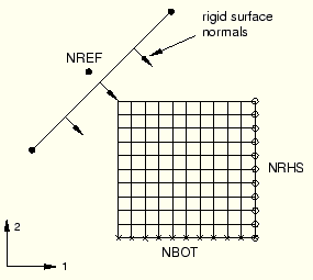
The node sets shown in Figure 4–10 are necessary to apply the loads and boundary conditions and to visualize output. Put the block elements in an element set called EALL, and put the rigid element in an element set called ERIGID. You could define the rigid body using either deformable elements, discrete rigid elements, or an analytical rigid surface. For purposes of this example we assume that you are using a single discrete rigid element. The reference node, which you should place in node set NREF, can be positioned anywhere; however, it is convenient to place it close to its rigid body.
We now review the model data associated with this problem, including the model description, block definition, rigid body definition, material properties, boundary conditions, amplitude definition, and surface definitions.
Model description
Since you will study several different meshes in this example, choose a model heading that describes the analysis as well as the mesh, such as the following:
*HEADING
Hourglassing example
10 X 10 regular mesh
SI Units (kg, m, s, N)
Defining the block
Ensure that the element type is CPE4R. Use the following section properties to give the block a thickness of 0.10 m and refer to a material named RUBBER:
*SOLID SECTION, ELSET=EALL, MATERIAL=RUBBER, CONTROLS=HGLASS
.10,
*SECTION CONTROLS, NAME=HGLASS, HOURGLASS=RELAX STIFFNESS
Defining the rigid body
Use a single rigid element (element type R2D2) to define the rigid body that compresses the block at a 45° angle. Make the surface large enough to compress the block by the required amount. The rigid element nodes must be separate from the nodes defining the block. Define the rigid element so that its positive normal points toward the rubber block. For two-dimensional rigid elements the positive normal direction is defined by a 90° counterclockwise rotation from the direction going from the first node defining the element to the second. Define a rigid body reference node that will control the motion of the rigid body. Use the following section properties to define the rigid body:
*RIGID BODY, ELSET=<element set name>, REF NODE=<node number>
Material properties
The block in this example is made of rubber and, thus, should be modeled using the hyperelastic material model. The hyperelastic constants are given in Pascals and are typical for a synthetic rubber. Refer to Chapter 5, “Materials,” for more information about defining hyperelastic materials.
*MATERIAL, NAME=RUBBER
** hyperelastic constants in Pa
*HYPERELASTIC, POLYNOMIAL, N=1
3.2E6, .8E6
** density is 1500 kg/m^3
*DENSITY
1500.,
Fixed boundary conditions
Fixed boundary conditions can be defined in either the model or the history part of the input file. Define roller boundary conditions on the bottom and right-hand side of the block. Fix the rigid body's rotational degree of freedom as well.
*BOUNDARY
NBOT, 2
NRHS, 1
NREF, 6
Amplitude definition
To gradually compress the rubber block by prescribing a nodal displacement at the rigid body reference node, you must first define the loading amplitude in the model definition. The prescribed displacements in the history definition will then refer to this loading amplitude. Define a smooth linear loading amplitude that has a value of zero at the start of the step (time 0.0 s) and a value of 1.0 at the end of the step (time 0.1 s), such as the following:
*AMPLITUDE, NAME=CRUSH, DEFINITION=SMOOTH STEP
0., 0., .1, 1.
Since the parameter DEFINITION was set equal to SMOOTH STEP in the above option, the first and second derivatives of the amplitude curve will be zero at the endpoints of the specified time interval. This promotes a smooth transition from one amplitude level to another. This parameter is commonly used to promote quasi-static response and is discussed further in “Smooth amplitude curves,” Section 7.2.1.
Surface definitions
Define surfaces on the side of the rigid element that will contact the block and on the exterior of the block. Since the normal of the rigid element points toward the rubber block, contact will occur on the rigid element's positive (SPOS) face.
*SURFACE, NAME=RIGID
ERIGID, SPOS
*SURFACE, NAME=SOLID
EALL,
The history data required for this simulation are discussed next, including the step definition, contact definitions, loading, and output requests.
Step definition
The following would be an appropriate heading for this step:
*STEP
Compress the rubber block
The goal is to compress the block slowly so that the dynamic effects are not dominant. Since this model is quite small, computer time is not an issue. For this case 0.1 s is a sufficiently large amount of time to compress the block in a nearly static manner. (Quasi-static analyses will be discussed in detail in Chapter 7, “Quasi-Static Analysis.”) Therefore, choose 0.1 s as the total time for the step.
*DYNAMIC, EXPLICIT
, 0.1
Contact definitions
Contact is discussed in detail in Chapter 6, “Contact.” Define the contact between the rigid body and the block using the following:
*CONTACT PAIR, INTERACTION=INTER
SOLID, RIGID
*SURFACE INTERACTION, NAME=INTER
Loading
The loading for this analysis is a displacement boundary condition imposed on the rigid body reference node. As the rigid body moves, it compresses the block. To move the rigid body a distance of 0.017 m at a 45° angle, impose equal displacement boundary conditions of 0.012 m in both the 1-direction and the negative 2-direction.
*BOUNDARY, TYPE=DISPLACEMENT, AMPLITUDE=CRUSH
NREF, 1, 1, .012
NREF, 2, 2, -.012
Output requests
You want to have an output database file created during the analysis so you can use ABAQUS/Viewer to postprocess the results. Write the preselected field data and the model energies as history data to the output database file. Add the following output requests to your input file:
*OUTPUT, FIELD, NUMBER INTERVAL=20, VARIABLE=PRESELECT
*OUTPUT, HISTORY, FREQUENCY=1
*ENERGY OUTPUT
ALLAE, ALLKE, ALLSE, ALLVD,
ALLFD, ALLWK, ETOTAL
Setting the FREQUENCY parameter on the *OUTPUT, HISTORY option equal to 1 causes history data to be written to the output database file every increment, permitting great detail for postprocessing. However, if many variables are chosen, the price of such detail can be a large output database file.
Indicate the end of a step with the option
*END STEPMake sure that this input option is the last option in your model.
After storing your input in a file called hourglass_square.inp, run the analysis using the following command:
abaqus job=hourglass_square
If the analysis does not complete, check the files hourglass_square.dat and hourglass_square.sta for error messages. Modify your input file to remove any error messages. If you still have trouble running the analysis, compare your input file to the one provided in “Hourglassing in a rubber block,” Section A.4.
Start ABAQUS/Viewer by typing
abaqus viewer odb=hourglass_squareat the operating system prompt.
Plotting the deformed model shape
To begin this exercise, plot the deformed model shape.
To plot the deformed model shape:
From the main menu bar, select Plot![]() Deformed Shape; or use the
Deformed Shape; or use the ![]() tool in the toolbox.
tool in the toolbox.
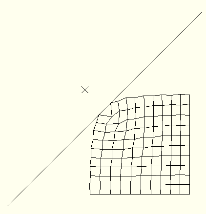
The deformed model plot appears in the current viewport as shown in Figure 4–11.
Looking closely at the deformation, you will notice that much of the mesh has a pattern of alternating trapezoids, which indicates that hourglassing is propagating through the mesh. The problem is most pronounced near the corner that is being pushed in. In this example the hourglassing pattern is severe enough that we can readily see the problem by looking at the deformed mesh. Usually, hourglassing is not a severe problem if it is not readily visible in the deformed mesh. A more quantitative approach is to look at the history of the artificial strain energy, which is primarily the energy dissipated to control hourglassing deformation. If the artificial strain energy is excessive, too much strain energy may be going into controlling hourglassing deformation.
Studying the artificial strain energy
To determine what is an excessive value of artificial strain energy, the most useful approach is to compare the artificial strain energy to the other internal energies. In this example the material is elastic; therefore, a comparison with the elastic strain energy is appropriate.
In ABAQUS/Explicit the variable ALLAE is the total energy dissipated as artificial strain energy and the variable ALLSE is the elastic, or recoverable, strain energy. ALLAE contains both viscous and elastic terms; however, since the viscous term is usually predominant, most of the energy that goes into artificial strain energy is non-recoverable. Look at the history of the artificial strain energy and the elastic strain energy in ABAQUS/Viewer to determine whether the amount of artificial strain energy is excessive in this problem.
To create history plots of the artificial and elastic strain energies:
In the Results Tree, expand the History Output container underneath the output database file named hourglass_square.odb.
Click mouse button 3 on the variable named Artificial strain energy: ALLAE for Whole Model and select Plot from the menu that appears.
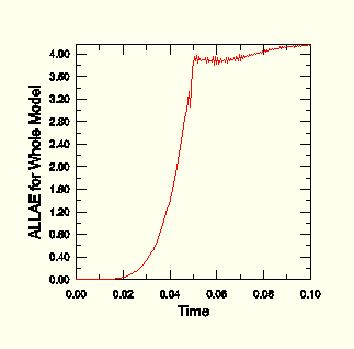
ABAQUS/Viewer plots the artificial strain energy history as shown in Figure 4–12.
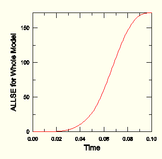
Click mouse button 3 on the variable named Strain energy: ALLSE for Whole Model and select Plot from the menu that appears.
ABAQUS/Viewer plots the elastic strain energy history as shown in Figure 4–13.
ABAQUS/Viewer allows you to create new X–Y data objects by performing operations on previously saved X–Y data objects. You will use this feature to create an X–Y data object that is the ratio of the artificial strain energy to the elastic strain energy versus time. Then, you will plot the ratio of artificial strain energy to elastic strain energy versus time.
To plot the ratio of artificial strain energy to elastic strain energy versus time:
In the Results Tree, click mouse button 3 on the history output variable ALLAE and select Save As from the menu that appears.
Name the X–Y data object ALLAE, and click OK.
Use a similar technique to save a data object containing the elastic strain energy (ALLSE). Name this data object ALLSE.
You are now ready to operate on the X–Y data objects.
In the Results Tree, double-click the XYData container.
The Create XY Data dialog box appears.
From the Create XY Data dialog box, select Operate on XY data and click Continue.
The Operate on XY Data dialog box appears.
From the XY Data field, double-click ALLAE.
“ALLAE” appears in the text field at the top of the dialog box.
From the Operators field, select the division symbol (/).
A division symbol appears following “ALLAE” in the text field at the top of the dialog box.
From the XY Data field, double-click ALLSE.
“ALLSE” is appended to the expression in the text field at the top of the dialog box.
Click Save As.
The Save XY Data As dialog box appears.
Name the data object AESE, and click OK.
A dialog box may appear warning that ABAQUS/Viewer detected an attempt to divide by zero. In this case the elastic strain energy is zero at time equal to zero, and you can safely click Dismiss. ABAQUS/Viewer sets the corresponding value to zero.
Dismiss the Operate on XY Data dialog box by clicking Cancel.
You are now ready to plot the ratio of artificial strain energy to elastic strain energy.
In the Results Tree, expand the XYData container.
The saved X–Y data objects are listed underneath.
Click mouse button 3 on the X–Y data object named AESE and select Plot from the menu that appears.
ABAQUS/Viewer plots the ratio of artificial strain energy to elastic strain energy versus time. By default, there is no title on the vertical axis. You will now add a title.
In the Results Tree, expand the XYPlots container.
The XYPlots-1 container appears underneath.
Click mouse button 3 on the XYPlots-1 container and select XY Plot Options from the menu that appears.
The XY Plot Options dialog box appears.
Click the Titles tab. From the Y-Axis options, change the title source to User-specified; then enter AESE for Whole Model for the title text.
Click OK.
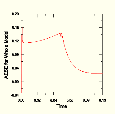
ABAQUS/Viewer creates the plot shown in Figure 4–14.
This plot shows that the ratio of artificial to elastic strain energy reaches a maximum of approximately 15% early in the analysis. You can ignore the transient values close to 0.00 s; these values are the result of dividing one very small number by another. After the maximum point little artificial energy is dissipated while elastic strain energy continues to increase, indicating that the hourglassing problem is not worsening. At the conclusion of the analysis, the ratio drops to approximately 2%. This plot confirms that for much of the analysis the ratio of energy dissipated as artificial strain energy to actual strain energy is well over 10%, while a general rule is that it is desirable to keep the ratio well below 5%. With the ratio of 10% we need to think about what is possibly causing the excessive artificial energy and how we can decrease the ratio to improve the results.
Understanding what is causing the mesh to hourglass so severely
To help understand what is causing the mesh to hourglass so severely, consider the deformed model shape near the time when the hourglassing is most severe. You must first determine when this occurs.
To determine when hourglassing is most severe:
From the main menu bar, select Tools![]() Query.
Query.
The Query dialog box appears.
From the Visualization Module Queries list, select Probe values; click OK.
The Probe Values dialog box appears.
Move the cursor over the curve, and locate the peak value on the curve.
As you move the mouse, notice that ABAQUS/Viewer displays the X–Y coordinates of the point currently under the cursor in the Probe Values field of the Probe Values dialog box. The peak value of the ratio of artificial strain energy to elastic strain energy occurs at 0.044 s.
Click Cancel to close the Probe Values dialog box.
Plot the deformed model shape in the vicinity of 0.044 s into the simulation to gain further insight into the source of the hourglassing.
To plot the deformed model shape near the time when hourglassing is most severe:
From the main menu bar, select Result![]() Step/Frame.
Step/Frame.
The Step/Frame dialog box appears.
In the Frame field of the Step/Frame dialog box, select the increment with a step time nearest to 0.044 s.
Click OK.
Subsequent deformed model plots will correspond to the increment you just selected.
From the main menu bar, select Plot![]() Deformed Shape; or use the
Deformed Shape; or use the ![]() tool in the toolbox.
tool in the toolbox.
ABAQUS/Viewer displays the deformed shape of the model. Turn on the display of node symbols.
From the main menu bar, select Options![]() Common; or use the
Common; or use the ![]() tool in the toolbox.
tool in the toolbox.
The Common Plot Options dialog box appears.
Click the Labels tab, and toggle on Show node symbols.
Click OK.
The deformed model plot is updated to reflect the selected deformed plot options.
Zoom in on the upper left corner of the mesh.
From the toolbar, click the ![]() tool and drag the mouse to select a rectangular region that encloses the upper left corner of the mesh.
tool and drag the mouse to select a rectangular region that encloses the upper left corner of the mesh.
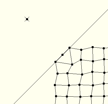
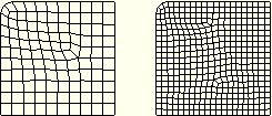
ABAQUS/Viewer zooms in on the selected region of the mesh as shown in Figure 4–15.
Click mouse button 2 to exit the box zoom mode.
The displaced mesh shows the classic hourglassing pattern, in which adjacent elements are alternating trapezoids. Several observations can be made. First, the corner element, which initially contacts the rigid body at a single node, is deformed excessively. Second, the hourglassing pattern is most severe in elements close to the corner element. Third, the hourglassing pattern appears to be more severe in the elements with free edges than in interior elements. Since these observations are based only on the displaced shape, they are somewhat subjective.
It appears that the hourglassing is seeded at the corner element, where the contact at a single node is similar to a concentrated force along the diagonal. Hourglassing propagates easily along the unconstrained boundaries of the block and along the diagonal. As the analysis progresses, the free boundaries become further constrained by contact with the rigid body, and the severity of the hourglassing decreases. Table 4–1 lists three common causes of hourglassing and remedies for the problem.
Table 4–1 Common causes and remedies of excessive hourglassing.
| Cause | Remedy |
|---|---|
| Concentrated force at a single node | Distribute the force among several nodes or apply a distributed load. |
| Boundary condition at a single node | Distribute the boundary constraint among several nodes. |
| Contact at a single node | Distribute the contact constraint among several nodes. |
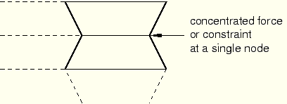
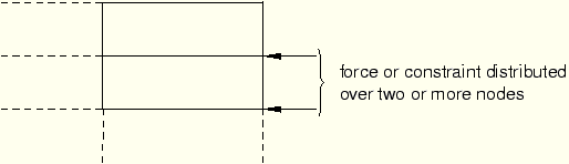
In summary, loads, boundary conditions, or contact constraints at a single node tend to promote hourglassing, as shown in Figure 4–16. On the other hand, distributing the load or constraint over two or more nodes greatly reduces hourglassing problems, as shown in Figure 4–17.
There are two specific changes we can make to the rubber block mesh to reduce hourglassing.
Refine the mesh, as mesh refinement always decreases hourglassing; or
Round the corner so that contact never occurs at only a single node. Distributing the contact constraint over several nodes removes the “seed” for the hourglassing deformation pattern.
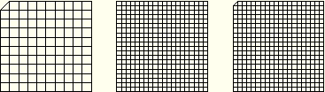
To illustrate the effects of refining the mesh and distributing the contact constraint over several nodes, we have created the three additional meshes shown in Figure 4–18.
Figure 4–18 From left to right: a coarse, flat-cornered mesh (mesh 2); a fine, square mesh (mesh 3); a fine, flat-cornered mesh (mesh 4).
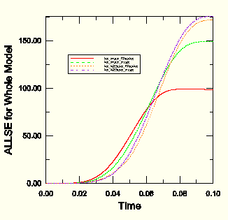
We study the quality of the results from these new meshes in the same manner as before, using X–Y plots of energy and deformed plots of the mesh. Figure 4–20 shows the elastic strain energy history using the original mesh and using the three new meshes. Since the block is compressed monotonically, it follows that the strain energy should increase monotonically as well, as the plot confirms. The maximum strain energy is lower in the models with the flat corner than in the models with the sharp corner because the flat-corner models contain less material at the corner and compressing less material stores less strain energy. With mesh refinement the differences decrease between the flat-corner and square mesh results.
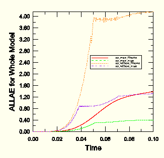
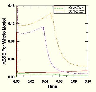
Figure 4–21 shows the histories of artificial strain energy for the four meshes, for which the trends are clear.
Mesh 1 (the coarse, square mesh) has by far the highest artificial strain energy; and mesh 3 (the fine, square mesh) has the next highest artificial strain energy, although its level is much lower than that of the coarse mesh. For each of these cases the artificial strain energy initially dissipates rapidly but eventually reaches a plateau and remains nearly constant. The rapid increase occurs while there is contact at only a single node; after two nodes come into contact, the highest artificial strain energy increases very little. This observation leads to the conclusion that the sooner two or more nodes are in contact, the sooner the hourglassing will diminish. From the beginning the flat-cornered meshes have two nodes in contact; thus, they do not show an initial plateau in the artificial strain energy. Even the coarse, flat-cornered mesh (mesh 2) has a lower artificial strain energy than the fine, square mesh, suggesting that distributing the contact forces between two nodes does more to decrease hourglassing than refining the mesh. Still lower in artificial strain energy is the fine, flat-cornered mesh whose advantages over the square mesh include mesh refinement and distributed contact forces.Figure 4–22 shows how the ratio of the dissipated artificial strain energy to elastic strain energy changes as the analysis progresses (the transient values close to 0.00 s are the result of dividing one very small number by another).
The trends are the same as for the artificial strain energy plots alone. The advantage of energy ratios is that they allow us to use a simple approximate rule to determine whether or not hourglassing is a problem. For both the coarse and fine square meshes the ratio, which is between 10% and 15% throughout the analysis, exceeds the 5% rule. Only after the rubber block becomes highly compressed does the ratio drop below 5%. For the flat-cornered meshes the ratio remains below 2% throughout the entire analysis, indicating that hourglassing is insignificant.For this example we showed the most basic way to distribute the corner contact forces by flattening the corner of the rubber block. While this approach clearly illustrates a remedy for excessive hourglassing, a more general approach would be to round the corner with a smooth fillet instead of replacing the corner element with a triangular element. A coarse, filleted mesh and a refined, filleted mesh are shown in Figure 4–23. Though their behavior is slightly more complicated than that of their flat-cornered counterparts, these meshes alleviate hourglassing problems in the same manner. Once more than one node is in contact at the corner, the hourglassing problem diminishes. The rounded meshes are somewhat more appealing for real engineering simulations because they allow a better representation of the physical problem.