The actual time taken for a physical process is called its natural time. Generally, it is safe to assume that performing an analysis in the natural time for a quasi-static process will produce accurate static results. After all, if the real-life event actually occurs in a natural time scale in which velocities are zero at the conclusion, a dynamic analysis should be able to capture the fact that the analysis has, in fact, achieved a steady state. You can increase the loading rate so that the same physical event occurs in less time as long as the solution remains nearly the same as the true static solution and dynamic effects remain insignificant.
For accuracy and efficiency quasi-static analyses require the application of loading that is as smooth as possible. Sudden, jerky movements cause stress waves, which can induce noisy or inaccurate solutions. Applying the load in the smoothest possible manner requires that the acceleration changes only a small amount from one increment to the next. If the acceleration is smooth, it follows that the changes in velocity and displacement are also smooth.
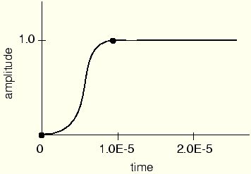
ABAQUS has a simple, built-in type of amplitude called SMOOTH STEP that automatically creates a smooth loading amplitude. When you define time-amplitude data pairs using *AMPLITUDE, DEFINITION=SMOOTH STEP, ABAQUS/Explicit automatically connects each of your data pairs with curves whose first and second derivatives are smooth and whose slopes are zero at each of your data points. Since both of these derivatives are smooth, you can apply a displacement loading with SMOOTH STEP using only the initial and final data points, and the intervening motion will be smooth. Using this type of loading amplitude allows you to perform a quasi-static analysis without generating waves due to discontinuity in the rate of applied loading. For example, for the following amplitude definition ABAQUS/Explicit creates the amplitude curve shown in Figure 7–2:
*AMPLITUDE, DEFINITION=SMOOTH STEP
0.0, 0.0, 1.0E-5, 1.0
Figure 7–2 Amplitude definition using *AMPLITUDE, DEFINITION=SMOOTH STEP.
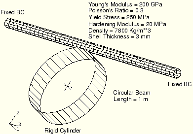
In a static analysis the lowest mode of the structure usually dominates the response. Knowing the frequency and, correspondingly, the period of the lowest mode, you can estimate the time required to obtain the proper static response. To illustrate the problem of determining the proper loading rate, consider the deformation of a side intrusion beam in a car door by a rigid cylinder, as shown in Figure 7–3. The actual test is quasi-static.
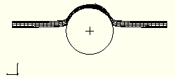
The response of the beam varies greatly with the loading rate. At an extremely high impact velocity of 400 m/s, the deformation in the beam is highly localized, as shown in Figure 7–4. To obtain a better quasi-static solution, consider the lowest mode.
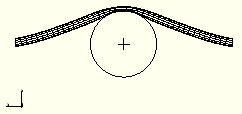
The frequency of the lowest mode is approximately 250 Hz, which corresponds to a period of 4 milliseconds. The natural frequencies can easily be calculated using the *FREQUENCY procedure in ABAQUS/Standard. To deform the beam by the desired 0.2 m in 4 milliseconds, the velocity of the cylinder is 50 m/s. While 50 m/s still seems like a high, impact velocity, the inertial forces become secondary to the overall stiffness of the structure, and the deformed shape—shown in Figure 7–5—indicates a much better quasi-static response. While the overall structural response appears to be what we expect as a quasi-static solution, it is usually desirable to increase the loading time to 10 times the period of the lowest mode to be certain that the solution is truly quasi-static. To improve the results even further, the velocity of the rigid cylinder could be ramped up gradually—for example, using a SMOOTH STEP amplitude definition—thereby easing the initial impact.Artificially increasing the speed of forming events is necessary to obtain an economical solution, but how large a speed-up can we impose and still obtain an acceptable static solution? If the deformation of the sheet metal blank corresponds to the deformed shape of the lowest mode, the time period of the lowest structural mode can be used as a guideline for forming speed. However, in forming processes the rigid dies and punches can constrain the punch in such a way that its deformation may not relate to the structural modes. In such cases a general recommendation is to limit punch speeds to less than 1% of the sheet metal wave speed. For typical processes the punch speed is on the order of 1 m/s, while the wave speed of steel is approximately 5000 m/s. This recommendation, therefore, suggests a factor of 50 as an upper bound on the speed-up of the punch velocity.
The suggested approach to determining an acceptable punch velocity involves running a series of analyses at various punch speeds in the range of 3 to 50 m/s. Perform the analyses in the order of fastest to slowest since the solution time is inversely proportional to the punch velocity. Examine the results of the analyses, and get a feel for how the deformed shapes, stresses, and strains vary with punch speed. Some indications of excessive punch speeds are unrealistic, localized stretching and thinning as well as the suppression of wrinkling. If you begin with a punch speed of, for example, 50 m/s, and decrease it from there, at some point the solutions will become similar from one punch speed to the next—an indication that the solutions are converging on a steady-state solution. As inertial effects become less significant, differences in simulation results also become less significant.
As the loading rate is increased artificially, it becomes more and more important to apply the loads in a gradual and smooth manner. For example, the simplest way to load the punch is to impose a constant velocity throughout the forming step. Such a loading causes a sudden impact load onto the sheet metal blank at the start of the analysis, which propagates stress waves through the blank and may produce undesired results. The effect of any impact load on the results becomes more pronounced as the loading rate is increased. Ramping up the punch velocity from zero using a SMOOTH STEP amplitude minimizes these adverse effects.
Springback
Springback is often an important part of a forming analysis because the springback analysis determines the shape of the final, unloaded part. While ABAQUS/Explicit is well-suited for forming simulations, springback poses some special difficulties. The main problem with performing springback simulations within ABAQUS/Explicit is the amount of time required to obtain a steady-state solution. Typically, the loads must be removed very carefully, and damping must be introduced to make the solution time reasonable. Fortunately, the close relationship between ABAQUS/Explicit and ABAQUS/Standard allows a much more efficient approach.
Since springback involves no contact and usually includes only mild nonlinearities, ABAQUS/Standard can solve springback problems much faster than ABAQUS/Explicit can. Therefore, the preferred approach to springback analyses is to import the completed forming model from ABAQUS/Explicit into ABAQUS/Standard. You must create an ABAQUS/Standard input file that will import the forming results and perform the springback analysis. Using the *IMPORT option within the ABAQUS/Standard input file, you specify the element sets that you wish to import. Usually, the entire deformable mesh is imported. The nodes, elements, and section properties are imported automatically, but you must redefine the materials and boundary conditions. Once the springback analysis is complete, you can import the model back into ABAQUS/Explicit to continue with another forming stage.