The interaction between contacting surfaces consists of two components: one normal to the surfaces and one tangential to the surfaces. The tangential component consists of the relative motion (sliding) of the surfaces and, possibly, frictional shear stresses. Each contact interaction can refer to a contact property that specifies a model for the interaction between the contacting surfaces. There are several contact interaction models available in ABAQUS; the default model is frictionless contact with no bonding.
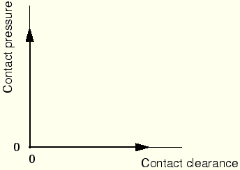
The distance separating two surfaces is called the clearance. The contact constraint is applied in ABAQUS when the clearance between two surfaces becomes zero. There is no limit in the contact formulation on the magnitude of contact pressure that can be transmitted between the surfaces. The surfaces separate when the contact pressure between them becomes zero or negative, and the constraint is removed. This behavior, referred to as “hard” contact, is summarized in the contact pressure-clearance relationship shown in Figure 12–4.
The dramatic change in contact pressure that occurs when a contact condition changes from “open” (a positive clearance) to “closed” (clearance equal to zero) sometimes makes it difficult to complete contact simulations in ABAQUS/Standard; the same is not true for ABAQUS/Explicit since iteration is not required for explicit methods. Some techniques to overcome difficulties with contact simulations are discussed later in this chapter. Other sources of information include “Common difficulties associated with contact modeling in ABAQUS/Standard,” Section 29.2.11 of the ABAQUS Analysis User's Manual; “Common difficulties associated with contact modeling using the contact pair algorithm in ABAQUS/Explicit,” Section 29.4.6 of the ABAQUS Analysis User's Manual; the “Contact in ABAQUS/Standard” lecture notes; and the “Advanced Topics: ABAQUS/Explicit” lecture notes.In addition to determining whether contact has occurred at a particular point, an ABAQUS analysis also must calculate the relative sliding of the two surfaces. This can be a very complex calculation; therefore, ABAQUS makes a distinction between analyses where the magnitude of sliding is small and those where the magnitude of sliding may be finite. It is much less expensive computationally to model problems where the sliding between the surfaces is small. What constitutes “small sliding” is often difficult to define, but a general guideline to follow is that problems where a point contacting a surface does not slide more than a small fraction of a typical element dimension can use the “small-sliding” approximation.
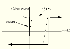
When surfaces are in contact, they usually transmit shear as well as normal forces across their interface. Thus, the analysis may need to take frictional forces, which resist the relative sliding of the surfaces, into account. Coulomb friction is a common friction model used to describe the interaction of contacting surfaces. The model characterizes the frictional behavior between the surfaces using a coefficient of friction, ![]() .
.
The default friction coefficient is zero. The tangential motion is zero until the surface traction reaches a critical shear stress value, which depends on the normal contact pressure, according to the following equation:
![]()
In ABAQUS/Standard the discontinuity between the two states—sticking or slipping—can result in convergence problems during the simulation. You should include friction in your ABAQUS/Standard simulations only when it has a significant influence on the response of the model. If your contact simulation with friction encounters convergence problems, one of the first modifications you should try in diagnosing the difficulty is to rerun the analysis without friction. In general, friction presents no additional computational difficulties for ABAQUS/Explicit.
Simulating ideal friction behavior can be very difficult; therefore, by default in most cases, ABAQUS uses a penalty friction formulation with an allowable “elastic slip,” shown by the dotted line in Figure 12–5. The “elastic slip” is the small amount of relative motion between the surfaces that occurs when the surfaces should be sticking. ABAQUS automatically chooses the penalty stiffness (the slope of the dotted line) so that this allowable “elastic slip” is a very small fraction of the characteristic element length. The penalty friction formulation works well for most problems, including most metal forming applications.
In those problems where the ideal stick-slip frictional behavior must be included, the “Lagrange” friction formulation can be used in ABAQUS/Standard and the kinematic friction formulation can be used in ABAQUS/Explicit. The “Lagrange” friction formulation is more expensive in terms of the computer resources used because ABAQUS/Standard uses additional variables for each surface node with frictional contact. In addition, the solution converges more slowly so that additional iterations are usually required. This friction formulation is not discussed in this guide.
Kinematic enforcement of the frictional constraints in ABAQUS/Explicit is based on a predictor/corrector algorithm. The force required to maintain a node's position on the opposite surface in the predicted configuration is calculated using the mass associated with the node, the distance the node has slipped, and the time increment. If the shear stress at the node calculated using this force is greater than ![]() , the surfaces are slipping, and the force corresponding to
, the surfaces are slipping, and the force corresponding to ![]() is applied. In either case the forces result in acceleration corrections tangential to the surface at the slave node and the nodes of the master surface facet that it contacts.
is applied. In either case the forces result in acceleration corrections tangential to the surface at the slave node and the nodes of the master surface facet that it contacts.
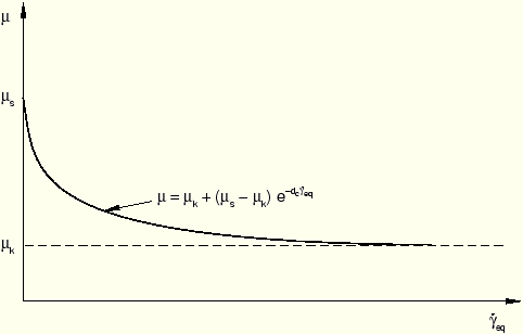
Often the friction coefficient at the initiation of slipping from a sticking condition is different from the friction coefficient during established sliding. The former is typically referred to as the static friction coefficient, and the latter is referred to as the kinetic friction coefficient. In ABAQUS an exponential decay law is available to model the transition between static and kinetic friction (see Figure 12–6). This friction formulation is not discussed in this guide.
In ABAQUS/Standard the inclusion of friction in a model adds unsymmetric terms to the system of equations being solved. If ![]() is less than about 0.2, the magnitude and influence of these terms are quite small and the regular, symmetric solver works well (unless the contact surface has high curvature). For higher coefficients of friction, the unsymmetric solver is invoked automatically because it will improve the convergence rate. The unsymmetric solver requires twice as much computer memory and scratch disk space as the symmetric solver. Large values of
is less than about 0.2, the magnitude and influence of these terms are quite small and the regular, symmetric solver works well (unless the contact surface has high curvature). For higher coefficients of friction, the unsymmetric solver is invoked automatically because it will improve the convergence rate. The unsymmetric solver requires twice as much computer memory and scratch disk space as the symmetric solver. Large values of ![]() generally do not cause any difficulties in ABAQUS/Explicit.
generally do not cause any difficulties in ABAQUS/Explicit.
The other contact interaction models available in ABAQUS depend on the analysis product and the algorithm used and may include adhesive contact behavior, softened contact behavior, fasteners (for example, spot welds), and viscous contact damping. These options are not discussed in this guide. Details about them can be found in the ABAQUS Analysis User's Manual.
Tie constraints are used to tie together two surfaces for the duration of a simulation. Each node on the slave surface is constrained to have the same motion as the point on the master surface to which it is closest. For a structural analysis this means the translational (and, optionally, the rotational) degrees of freedom are constrained.
ABAQUS uses the undeformed configuration of the model to determine which slave nodes are tied to the master surface. By default, all slave nodes that lie within a given distance of the master surface are tied. The default distance is based on the typical element size of the master surface. This default can be overridden in one of two ways: by specifying the distance within which slave nodes must lie from the master surface to be constrained or by specifying the name of a set containing the nodes that will be constrained.
Slave nodes can also be adjusted so that they lie exactly on the master surface. If slave nodes have to be adjusted by distances that are a large fraction of the length of the side of the element (to which the slave node is attached), the element can become severely distorted; avoid large adjustments if possible.
Tie constraints are particularly useful for rapid mesh refinement between dissimilar meshes.