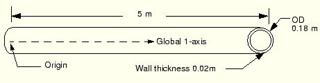
In this example you will study the vibrational frequencies of a 5 m long section of a piping system. The pipe is made of steel and has an outer diameter of 18 cm and a 2 cm wall thickness (see Figure 11–5).
It is clamped firmly at one end and can move only axially at the other end. This 5 m portion of the piping system may be subjected to harmonic loading at frequencies up to 50 Hz. The lowest vibrational mode of the unloaded structure is 40.1 Hz, but this value does not consider how the loading applied to the piping structure may affect its response. To ensure that the section does not resonate, you have been asked to determine the magnitude of the in-service load that is required so that its lowest vibrational mode is higher than 50 Hz. You are told that the section of pipe will be subjected to axial tension when in service. Start by considering a load magnitude of 4 MN.The lowest vibrational mode of the pipe will be a sine wave deformation in any direction transverse to the pipe axis because of the symmetry of the structure's cross-section. You use three-dimensional beam elements to model the pipe section.
The analysis requires a natural frequency extraction. Thus, you will use ABAQUS/Standard as your analysis product.
Create the model for this example using ABAQUS/CAE. A Python script is provided in “Vibration of a piping system,” Section A.11. When this script is run through ABAQUS/CAE, it creates the complete analysis model for this problem. Run this script if you encounter difficulties following the instructions given below or if you wish to check your work. Instructions on how to fetch and run the script are given in Appendix A, “Example Files.”
If you do not have access to ABAQUS/CAE or another preprocessor, the input file required for this problem can be created manually, as discussed in “Example: vibration of a piping system,” Section 10.3 of Getting Started with ABAQUS/Standard: Keywords Version.
Part geometry
Create a three-dimensional, deformable, planar wire part. (Remember to use an approximate part size that is slightly larger than the largest dimension in your model.) Name the part Pipe, and use the Create Lines: Connected tool to sketch a horizontal line of length 5.0 m. Dimension the sketch as needed to ensure that the length is specified precisely.
Material and section properties
The pipe is made of steel with a Young's modulus of 200 × 109 Pa and a Poisson's ratio of 0.3. Create a linear elastic material named Steel with these properties. You must also define the density of the steel material (7800 kg/m3) because eigenmodes and eigenfrequencies will be extracted in this simulation and a mass matrix is needed for this type of procedure.
Next, create a Pipe profile. Name the profile PipeProfile, and specify an outer radius of 0.09 m and a wall thickness of 0.02 m for the pipe.
Create a Beam section named PipeSection. In the Edit Beam Section dialog box, specify that section integration will be performed during the analysis and assign material Steel and profile PipeProfile to the section definition.
Finally, assign section PipeSection to the pipe. In addition, define the approximate ![]() -direction as the vector (0.0, 0.0, –1.0) (the default). In this model the actual
-direction as the vector (0.0, 0.0, –1.0) (the default). In this model the actual ![]() -vector will coincide with this approximate vector.
-vector will coincide with this approximate vector.
Assembly and sets
Create a dependent instance of the part named Pipe. For convenience, create geometry sets that contain the vertices at the left and right ends of the pipe and name them Left and Right, respectively. These regions will be used later to assign loads and boundary conditions to the model.
Steps
In this simulation you need to investigate the eigenmodes and eigenfrequencies of the steel pipe section when a 4 MN tensile load is applied. Therefore, the analysis will be split into two steps:
| Step 1. General step: | Apply a 4 MN tensile force. |
| Step 2. Linear perturbation step: | Calculate modes and frequencies. |
You need to calculate the eigenmodes and eigenfrequencies of the pipe in its loaded state. Thus, create a second analysis step using the linear perturbation frequency extraction procedure. Name the step Frequency I, and give it the following description: Extract modes and frequencies. Although only the first (lowest) eigenmode is of interest to you, extract the first eight eigenmodes for the model. Since a small number of eigenvalues is requested, use the subspace iteration eigensolver.
Output requests
The default output database output requests created by ABAQUS/CAE for each step will suffice; you do not need to create any additional output database output requests.
To request output to the restart file, select Output![]() Restart Requests from the main menu bar of the Step module. For the step labeled Pull I, write data to the restart file every 10 increments; for the step labeled Frequency I, write data to the restart file every increment.
Restart Requests from the main menu bar of the Step module. For the step labeled Pull I, write data to the restart file every 10 increments; for the step labeled Frequency I, write data to the restart file every increment.
Loads and boundary conditions
In the first step create a load named Force that applies a 4 × 10⁶ N tensile force to the right end of the pipe section such that it deforms in the positive axial (global 1) direction. Forces are applied, by default, in the global coordinate system.
The pipe section is clamped at its left end. It is also clamped at the other end; however, the axial force must be applied at this end, so only degrees of freedom 2 through 6 (U2, U3, UR1, UR2, and UR3) are constrained. Apply the appropriate boundary conditions to sets Left and Right in the first step.
In the second step you require the natural frequencies of the extended pipe section. This does not involve the application of any perturbation loads, and the fixed boundary conditions are carried over from the previous general step. Therefore, you do not need to specify any additional loads or boundary conditions in this step.
Mesh and job definition
Seed and mesh the pipe section with 30 uniformly spaced second-order, pipe elements (PIPE32).
Before continuing, rename the model to Original. This model will later form the basis of the model used in the example discussed in “Example: restarting the pipe vibration analysis,” Section 11.5.
Create a job named Pipe with the following description: Analysis of a 5 meter long pipe under tensile load.
Save your model in a model database file, and submit the job for analysis. Monitor the solution progress; correct any modeling errors and investigate the source of any warning messages, taking corrective action as necessary.
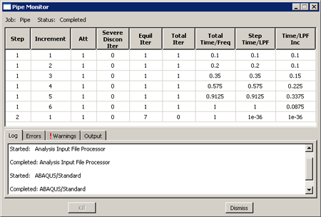
Check the Job Monitor as the job is running. When the analysis completes, its contents will look similar to Figure 11–6.
Both steps are shown, and the time associated with the linear perturbation step (Step 2) is very small: the frequency extraction procedure, or any linear perturbation procedure, does not contribute to the general loading history of the model.
Enter the Visualization module, and open the output database file, Pipe.odb, created by this job.
Deformed shapes from the linear perturbation steps
The Visualization module automatically uses the last available frame on the output database file. The results from the second step of this simulation are the natural mode shapes of the pipe and the corresponding natural frequencies. Plot the first mode shape.
To plot the first mode shape:
From the main menu bar, select Result![]() Step/Frame.
Step/Frame.
The Step/Frame dialog box appears.
Select step Frequency I and frame Mode 1.
Click OK.
From the main menu bar, select Plot![]() Deformed Shape.
Deformed Shape.
Click the ![]() tool in the toolbox to allow multiple plot states in the viewport; then click the
tool in the toolbox to allow multiple plot states in the viewport; then click the ![]() tool or select Plot
tool or select Plot![]() Undeformed Shape to add the undeformed shape plot to the existing deformed plot in the viewport.
Undeformed Shape to add the undeformed shape plot to the existing deformed plot in the viewport.
Include node symbols on both plots (the superimpose options control the appearance of the undeformed shape when multiple plot states are displayed). Change the color of the node symbols to green and the symbol shape to a solid circle.
Click the auto-fit tool ![]() so that the entire plot is rescaled to fit in the viewport.
so that the entire plot is rescaled to fit in the viewport.
The default view is isometric. Try rotating the model to find a better view of the first eigenmode, similar to that shown in Figure 11–7.
Figure 11–7 First and second eigenmode shapes of the pipe section under the tensile load (the modes lie in planes orthogonal to each other).
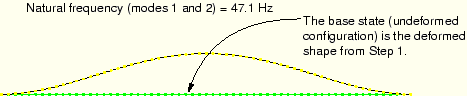
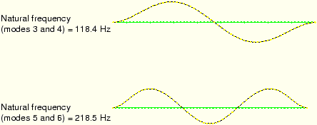
Since this is a linear perturbation step, the undeformed shape is the shape of the structure in the base state. This makes it easy to see the motion relative to the base state. Use the Frame Selector to plot the other mode shapes. You will discover that this model has many repeated eigenmodes. This is a result of the symmetric nature of the pipe's cross-section, which yields two eigenmodes for each natural frequency, corresponding to the 1–2 and 1–3 planes. The second eigenmode shape is shown in Figure 11–7. Some of the higher vibrational mode shapes are shown in Figure 11–8.
Figure 11–8 Shapes of eigenmodes 3 through 6; corresponding mode shapes lie in planes orthogonal to each other.
The natural frequency associated with each eigenmode is reported in the plot title. The lowest natural frequency of the pipe section when the 4 MN tensile load is applied is 47.1 Hz. The tensile loading has increased the stiffness of the pipe and, thus, increased the vibrational frequencies of the pipe section. This lowest natural frequency is within the frequency range of the harmonic loads; therefore, resonance of the pipe may be a problem when it is used with this loading.
You, therefore, need to continue the simulation and apply additional tensile load to the pipe section until you find the magnitude that raises the natural frequency of the pipe section to an acceptable level. Rather than repeating the analysis and increasing the applied axial load, you can use the restart capability in ABAQUS to continue the load history of a prior simulation in a new analysis.