This example demonstrates some of the fundamental ideas in explicit dynamics described earlier in Chapter 2, “ABAQUS Basics.” It also illustrates stability limits and the effect of mesh refinement and materials on the solution time.
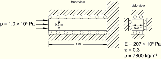
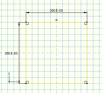
The bar has the dimensions shown in Figure 9–1.
To make the problem a one-dimensional strain problem, all four lateral faces are on rollers; thus, the three-dimensional model simulates a one-dimensional problem. The material is steel with the properties shown in Figure 9–1. The free end of the bar is subjected to a blast load with a magnitude of 1.0 × 10⁵ Pa, as shown in Figure 9–2, in which the duration of the blast load is 3.88 × 10⁻⁵ s.In this section we discuss how to use ABAQUS/CAE to create the model for this simulation. A Python script is provided in “Stress wave propagation in a bar,” Section A.7. When the script is run in ABAQUS/CAE, it creates the complete analysis model for this problem. Run the script if you encounter difficulties following the instructions given below or if you wish to check your work. Instructions on how to fetch and run the script are given in Appendix A, “Example Files.”
If you do not have access to ABAQUS/CAE or another preprocessor, the input file that defines this problem can be created manually, as discussed in “Example: stress wave propagation in a bar,” Section 3.4 of Getting Started with ABAQUS/Explicit: Keywords Version.
Defining the model geometry
In this example you will create a three-dimensional, deformable body with a solid, extruded base feature. You will first sketch the two-dimensional profile of the bar and then extrude it.
To create a part:
Create a new part named Bar, and accept the default settings of a three-dimensional, deformable body and a solid, extruded base feature in the Create Part dialog box. Use an approximate size of 0.50 for the model.
Use the dimensions given in Figure 9–3 to sketch the cross-section of the bar.
The following possible approach can be used:Create an arbitrary rectangle using the Create Lines: Rectangle tool.
Dimension the sketch so that the cross section is 0.20 m high × 0.20 m wide.
Click Done in the prompt area when you are finished sketching the profile.
The Edit Base Extrusion dialog box appears. To complete the part definition, you must specify the distance over which the profile will be extruded.
In the dialog box, enter an extrusion depth of 1.0 m.
Save your model in a model database file named Bar.cae.
Defining the material and section properties
Create a single linear elastic material named Steel with a mass density of 7800 kg/m3, a Young's modulus of 207E9 Pa, and a Poisson's ratio of 0.3.
Create a solid, homogeneous section definition named BarSection. Accept Steel as the material and 1 as the Plane stress/strain thickness.
Assign the section definition BarSection to the entire part.
Creating an assembly
Create an instance of the bar. The model is oriented by default so that the global 3-axis lies along the length of the bar.
Creating geometry sets and surfaces
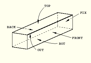
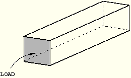
Create the geometry sets TOP, BOT, FRONT, BACK, FIX, and OUT as shown in Figure 9–4. (The set OUT contains the edge shown in bold in Figure 9–4.) Create the surface named LOAD shown in Figure 9–5. These regions will be used later for the application of loads and boundary conditions, as well as for the definition of output requests.
Defining steps
Create a single dynamic, explicit step named BlastLoad. Enter Apply pressure load pulse as the step description, and set the Time period to 2.0E-4 s. In the Edit Step dialog box, click the Other tab. To keep the stress wave as sharp as possible, set the Quadratic bulk viscosity parameter (discussed in “Bulk viscosity,” Section 9.5.1) to zero.
Specifying output requests
Edit the default field output request so that preselected field data are written to the output database at four equally spaced intervals for the step BlastLoad.
Delete the existing default history output request, and create a new set of history output requests. In the Create History Output dialog box, accept the default name of H-Output-1 and select the BlastLoad step. Click Continue. Click the arrow next to the Domain field, select Set, and select OUT. In the Output Variables section, click on the triangle to the left of Stresses. Click on the triangle to the left of S, Stress components and invariants, and toggle on the S33 variable, which is the component of stress in the axial direction of the bar. Specify that output be saved at every 1.0E-6 s.
Prescribing boundary conditions
Create a boundary condition named Fix right end, and constrain the right end of the bar (geometry set FIX) in all three directions (see Figure 9–1). Create additional boundary conditions to constrain the top, bottom, front, and back faces in the directions normal to these faces (the 1-direction for sets FRONT and BACK and the 2-direction for sets TOP and BOT).
Defining the load history
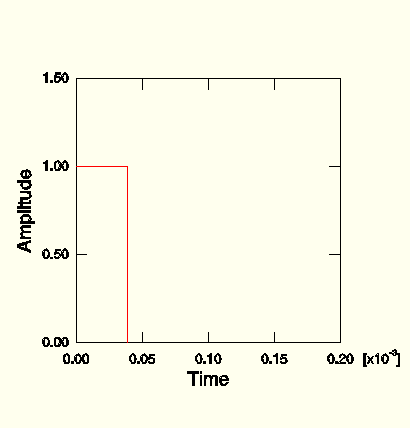
The blast load is applied at its maximum value instantaneously and is held constant for 3.88 × 10⁻⁵ s. Then the load is suddenly removed and held constant at zero. Create an amplitude definition named Blast using the data shown in Figure 9–6. For this problem the pressure load at any given time is the specified magnitude of the pressure load times the value interpolated from the amplitude curve.
Create a pressure load named Blast load, and select BlastLoad as the step in which it will be applied. Apply the load to the surface LOAD. Select Uniform for the distribution, specify a value of 1.0E5 Pa for the load magnitude, and select Blast for the amplitude.
Creating a mesh
Using the material properties (neglecting Poisson's ratio), we can calculate the wave speed of the material using the equations introduced earlier.
![]()
Seed the instance with a target global element size of 0.02. Select C3D8R as the element type, and mesh the instance.
Note: The proposed mesh density exceeds the model size limits of the ABAQUS Student Edition. If you are using this product, specify one of the following:
A global element size of 0.04.
A 50 × 3 × 3 mesh.
A 25 × 5 × 5 mesh.
Creating, running, and monitoring a job
Create a job named Bar, and enter Stress wave propagation in a bar (SI units) for the job description. Submit the job, and monitor the results. If any errors are encountered, correct the model and rerun the simulation. Be sure to investigate the cause of any warning messages and take appropriate action; recall that some warning messages can be ignored safely while others require corrective action.
The status (.sta) file
You can also look at the status file, Bar.sta, to monitor the job progress. It contains information about moments of inertia, followed by information concerning the stability limit. The 10 elements with the lowest stable time limits are listed in rank order.
    Most critical elements :
     Element number   Rank    Time increment   Increment ratio
     (Instance name)
    ----------------------------------------------------------
         502          1       1.819457E-06      1.000000E+00
    BAR-1
         503          2       1.819457E-06      1.000000E+00
    BAR-1
         504          3       1.819457E-06      1.000000E+00
    BAR-1
         505          4       1.819457E-06      1.000000E+00
    BAR-1
         506          5       1.819457E-06      1.000000E+00
    BAR-1
         507          6       1.819457E-06      1.000000E+00
    BAR-1
         508          7       1.819457E-06      1.000000E+00
    BAR-1
         509          8       1.819457E-06      1.000000E+00
    BAR-1
         522          9       1.819457E-06      1.000000E+00
    BAR-1
         523         10       1.819457E-06      1.000000E+00
    BAR-1
The status file continues with information about the progress of the solution. The information that follows also appears in the Job Monitor. STEP 1 ORIGIN 0.00000E+00
Total memory used for step 1 is approximately 7.2 megabytes.
Global time estimation algorithm will be used.
Scaling factor : 1.0000
Variable mass scaling factor at zero increment: 1.0000
STEP TOTAL CPU STABLE CRITICAL KINETIC
INCREMENT TIME TIME TIME INCREMENT ELEMENT ENERGY
0 0.000E+00 0.000E+00 00:00:00 1.819E-06 502 0.000E+00
INSTANCE WITH CRITICAL ELEMENT: BAR-1
ODB Field Frame Number 0 of 4 requested intervals at increment zero.
6 1.092E-05 1.092E-05 00:00:00 1.819E-06 502 4.126E-05
12 2.183E-05 2.183E-05 00:00:00 1.819E-06 522 8.715E-05
17 3.431E-05 3.431E-05 00:00:00 2.919E-06 502 1.380E-04
21 4.596E-05 4.596E-05 00:00:00 2.902E-06 502 1.660E-04
23 5.176E-05 5.176E-05 00:00:00 2.896E-06 502 1.648E-04
ODB Field Frame Number 1 of 4 requested intervals at 5.176230E-05
27 6.333E-05 6.333E-05 00:00:00 2.885E-06 502 1.616E-04
31 7.485E-05 7.485E-05 00:00:00 2.876E-06 622 1.585E-04
.
.
. In the Model Tree, click mouse button 3 on the job named Bar and select Results from the menu that appears to enter the Visualization module and automatically open the output database (.odb) file created by this job. Alternatively, from the Module list located under the toolbar, select Visualization to enter the Visualization module; open the .odb file by selecting File![]() Open from the main menu bar and double-clicking on the appropriate file.
Open from the main menu bar and double-clicking on the appropriate file.
Plotting the stress along a path
We are interested in looking at how the stress distribution along the length of the bar changes with time. To do so, we will look at the stress distribution at three different times throughout the course of the analysis.
Create a curve of the variation of the stress in the 3-direction (S33) along the center of the bar for each of the first three frames of the output database file. To create these plots, you first need to define a straight path along the center of the bar.
To create a point list path along the center of the bar:
In the Results Tree, double-click Paths.
The Create Path dialog box appears.
Name the path Center. Select Point list as the path type, and click Continue.
The Edit Point List Path dialog box appears.
In the Point Coordinates table, enter the coordinates of the centers of both ends of the bar. For example, if you generated the geometry and mesh using the procedure described earlier, the table entries are 0, 0, 1 and 0, 0, 0. (This input specifies a path from the point (0, 0, 1) to the point (0, 0, 0), as defined in the global coordinate system of the model.)
When you have finished, click OK to close the Edit Point List Path dialog box.
To save X–Y plots of stress along the path at three different times:
In the Results Tree, double-click XYData.
The Create XY Data dialog box appears.
Choose Path as the X–Y data source, and click Continue.
The XY Data from Path dialog box appears with the path that you created visible in the list of available paths. If the undeformed model shape is currently displayed, the path you select is highlighted in the plot.
Toggle on Include intersections under Point locations.
Accept True distance as the selection in the X Values portion of the dialog box.
Click Field Output in the Y Values portion of the dialog box to open the Field Output dialog box.
Select the S33 stress component, and click OK.
The field output variable in the XY Data from Path dialog box changes to indicate that stress data in the 3-direction (S33) will be created.
Note: ABAQUS/CAE may warn you that the field output variable will not affect the current image. Leave the plot state As is, and click OK to continue.
Click Step/Frame in the Y Values portion of the XY Data from Path dialog box.
In the Step/Frame dialog box that appears, choose frame 1, which is the second of the five recorded frames. (The first frame listed, frame 0, is the base state of the model at the beginning of the step.) Click OK.
The Y Values portion of the XY Data from Path dialog box changes to indicate that data from Step 1, frame 1 will be created.
To save the X–Y data, click Save As.
The Save XY Data As dialog box appears.
Name the X–Y data S33_T1, and click OK.
S33_T1 appears in the XYData container of the Results Tree.
Repeat Steps 7 through 9 to create X–Y data for frames 2 and 3. Name the data sets S33_T2 and S33_T3, respectively.
To close the XY Data from Path dialog box, click Cancel.
To plot the stress curves:
In the XYData container, drag the cursor to select all three X–Y data sets.
Click mouse button 3, and select Plot from the menu that appears.
ABAQUS/CAE plots the stress in the 3-direction along the center of the bar for frames 1, 2, and 3, corresponding to approximate simulation times of 5 × 10⁻⁵ s, 1 × 10⁻⁴ s, and 1.5 × 10⁻⁴ s, respectively.
To customize the X–Y plot:
In the Results Tree, expand the XYPlots container. Click mouse button 3 on XYPlot-1, and select XY Plot Options from the menu that appears.
The XY Plot Options dialog box appears.
Click the Tick Marks tab.
The Tick Marks options become available.
Specify that the Y-axis major tick marks occur at 20E3 s increments.
For both the X-axis and Y-axis minor tick mark options, specify zero minor tick marks between each major tick mark interval.
You can also customize the axis titles.
Click the Titles tab to make the Titles options available.
In the X-Axis area, select a User-specified title source. In the Title text field, enter Distance along bar (m).
In the Y-Axis area, specify Stress - S33 (Pa) as the Y-axis title.
Click OK to apply the customized X–Y plot parameters and to close the XY Plot Options dialog box.
To customize the appearance of the curves in the X–Y plot:
In the Results Tree, expand the XYPlot-1 container. Click mouse button 3 on Curve, and select XY Curve Options from the menu that appears.
The XY Curve Options dialog box appears.
In the XY Data field, select S33_T2.
Choose the dotted line style for the S33_T2 curve, and click Apply.
The S33_T2 curve becomes dotted.
Repeat Steps 2 and 3 to make the S33_T3 curve dashed.
Close the XY Curve Options dialog box.
The customized plot appears in Figure 9–8.
We can see that the length of the bar affected by the stress wave is approximately 0.2 m in each of the three curves. This distance should correspond to the distance that the blast wave travels during its time of application, which can be checked by a simple calculation. If the length of the wave front is 0.2 m and the wave speed is 5.15 × 10³ m/s, the time it takes for the wave to travel 0.2 m is 3.88 × 10⁻⁵ s. As expected, this is the duration of the blast load that we applied. The stress wave is not exactly square as it passes along the bar. In particular, there is “ringing” or oscillation of the stress behind the sudden changes in stress. Linear bulk viscosity, discussed later in this chapter, damps the ringing so that it does not affect the results adversely.
Creating a history plot
Another way to study the results is to view the time history of stress at three different points within the bar; for example, at distances of 0.25 m, 0.50 m, and 0.75 m from the loaded end of the bar. To do this, we must first determine the labels of the elements located at these positions. An easy way to accomplish this is to query the elements in a display group consisting of the elements along the edge of the bar (set OUT).
To create and plot a display group and query the element labels:
In the Results Tree, expand the Element Sets container underneath the output database file named Bar.odb. Click mouse button 3 on the set named OUT, and select Replace from the menu that appears.
To save this group, double-click Display Groups in the Results Tree; or use the ![]() tool in the toolbar.
tool in the toolbar.
The Create Display Group dialog box appears.
In the Create Display Group dialog box, click Save As and enter History plot as the name for your display group.
Click Dismiss to close the Create Display Group dialog box.
This display group now appears underneath the Display Groups container in the Results Tree.
From the main menu bar, select Tools![]() Query; or use the
Query; or use the ![]() tool in the toolbar.
tool in the toolbar.
In the Query dialog box that appears, select Element and click OK.
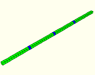
Click on the elements shaded in Figure 9–9 (every 13th element along the bar). The element ID (label) appears in the prompt area (and also in the message area). Make note of the element labels for the three shaded elements.
To plot the stress history:
In the Results Tree, expand the sub-containers underneath History Output.
Select the stress data in the 3-direction (S33) for the three elements you have identified (again, every 13th element). Use [Ctrl]+Click to select multiple X–Y data sets.
Click mouse button 3, and select Plot from the menu that appears.
ABAQUS/CAE displays an X–Y plot of the longitudinal stress in each element versus time.
Click Dismiss to close the dialog box.
As before, you can customize the appearance of the plot.
To customize the X–Y plot:
In the Results Tree, expand the XYPlots container. Click mouse button 3 on XYPlot-1, and select XY Plot Options from the menu that appears.
The XY Plot Options dialog box appears.
Click the Titles tab.
The Titles options become available.
In the X-axis area, specify Total time (s) as the X-axis title.
Click OK to apply the customized X–Y plot options and to close the dialog box.
To customize the appearance of the curves in the X–Y plot:
In the Results Tree, expand the XYPlot-1 container. Click mouse button 3 on Curve, and select XY Curve Options from the menu that appears.
The XY Curve Options dialog box appears.
In the XY Data field, select the temporary X–Y data label that corresponds to the element closest to the free end of the bar. (Of the elements in this set, this one is affected first by the stress wave.)
Select a User-specified legend source.
In the Legend text field, enter S33-0.25.
Click Apply.
In the XY Data field, select the temporary X–Y data label that corresponds to the element in the middle of the bar. (This is the element affected next by the stress wave.)
Specify S33-0.5 as the curve legend text, and change the curve style to dotted.
Click Apply.
In the XY Data field, select the temporary X–Y data label that corresponds to the element closest to the fixed end of the bar. (This is the element affected last by the stress wave.)
Specify S33-0.75 as the curve legend text, and change the curve style to dashed.
Click OK to apply your changes and to close the dialog box.
The customized plot appears in Figure 9–10.
In the history plot we can see that stress at a given point increases as the stress wave travels through the point. Once the stress wave has passed completely through the point, the stress at the point oscillates about zero.
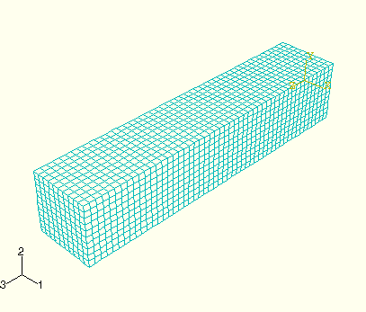
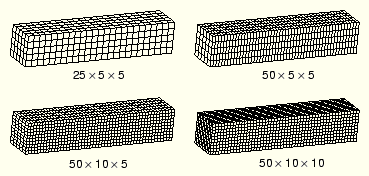
In “Automatic time incrementation and stability,” Section 9.3, we discussed how mesh refinement affects the stability limit and the CPU time. Here we will illustrate this effect with the wave propagation problem. We began with a reasonably refined mesh of square elements with 50 elements along the length and 10 elements in each of the two transverse directions. For illustrative purposes, we will now use a coarse mesh of 25 × 5 × 5 elements and observe how refining the mesh in the various directions changes the CPU time. The four meshes are shown in Figure 9–11.
Table 9–1 shows how the CPU time (normalized with respect to the coarse mesh model result) changes with mesh refinement for this problem. The first half of the table provides the expected results, based on the simplified stability equations presented in this guide; the second half of the table provides the results obtained by running the analyses in ABAQUS/Explicit on a desktop workstation.
Table 9–1 Mesh refinement and solution time.
| Mesh | Simplified Theory | Actual | ||||
|---|---|---|---|---|---|---|
| Number of Elements | CPU Time (s) | Max | Number of Elements | Normalized CPU Time | ||
| 25 × 5 × 5 | A | B | C | 6.06e-6 | 625 | 1 |
| 50 × 5 × 5 | A/2 | 2B | 4C | 3.14e-6 | 1250 | 4 |
| 50 × 10 × 5 | A/2 | 4B | 8C | 3.12e-6 | 2500 | 8.33 |
| 50 × 10 × 10 | A/2 | 8B | 16C | 3.11e-6 | 5000 | 16.67 |
For the theoretical results we choose the coarsest mesh, 25 × 5 × 5, as the base state, and we define the stable time increment, the number of elements, and the CPU time as variables A, B, and C, respectively. As the mesh is refined, two things happen: the smallest element dimension decreases, and the number of elements in the mesh increases. Each of these effects increases the CPU time. In the first level of refinement, the 50 × 5 × 5 mesh, the smallest element dimension is cut in half and the number of elements is doubled, increasing the CPU time by a factor of four over the previous mesh. However, further doubling the mesh to 50 × 10 × 5 does not change the smallest element dimension; it only doubles the number of elements. Therefore, the CPU time increases by only a factor of two over the 50 × 5 × 5 mesh. Further refining the mesh so that the elements are uniform and square in the 50 × 10 × 10 mesh again doubles the number of elements and the CPU time.
This simplified calculation predicts quite well the trends of how mesh refinement affects the stable time increment and CPU time. However, there are reasons why we did not compare the predicted and actual stable time increment values. First, recall that we made the approximation that the stable time increment is
![]()
The same wave propagation analysis performed on different materials would take different amounts of CPU time, depending on the wave speed of the material. For example, if we were to change the material from steel to aluminum, the wave speed would change from 5.15 × 10³ m/s to