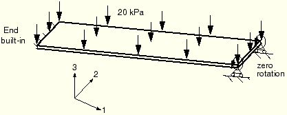
This example is a continuation of the linear skew plate simulation described in Chapter 5, “Using Shell Elements,” and shown in Figure 8–11.
Having already simulated the linear response of the plate in ABAQUS/Standard, you will now reanalyze it in ABAQUS/Standard including the effects of geometric nonlinearity. The results from the linear simulation indicated that nonlinear effects may be important for this problem. With the results of this analysis, you will now be able to judge whether this is true or not.If you wish, you can follow the guidelines at the end of this example to extend the simulation to perform a dynamic analysis using ABAQUS/Explicit.
A Python script is provided in “Nonlinear skew plate,” Section A.6. When this script is run through ABAQUS/CAE, it creates the complete analysis model for this problem. Run this script if you encounter difficulties following the instructions given below or if you wish to check your work. Instructions on how to fetch and run the script are given in Appendix A, “Example Files.”
If you do not have access to ABAQUS/CAE or another preprocessor, the input file required for this problem can be created manually, as discussed in “Example: nonlinear skew plate,” Section 7.4 of Getting Started with ABAQUS/Standard: Keywords Version.
Open the model database file SkewPlate.cae. Copy the model named Linear to a model named Nonlinear.
For the Nonlinear skew plate model, you will include nonlinear geometric effects as well as change the output requests.
Defining the step
In the Model Tree, double-click the Apply Pressure step underneath the Steps container to edit the step definition. In the Basic tabbed page of the Edit Step dialog box, toggle on Nlgeom to include geometric nonlinearity effects, and ensure the time period for the step is set to 1.0. In the Incrementation tabbed page, set the initial increment size to 0.1. The default maximum number of increments is 100; ABAQUS may use fewer increments than this upper limit, but it will stop the analysis if it needs more.
You may wish to change the description of the step to reflect that it is now a nonlinear analysis step.
Output control
In a linear analysis ABAQUS solves the equilibrium equations once and calculates the results for this one solution. A nonlinear analysis can produce much more output because results can be requested at the end of each converged increment. If you do not select the output requests carefully, the output files become very large, potentially filling the disk space on your computer.
As noted earlier, output is available in four different files:
the output database (.odb) file, which contains data in a neutral binary format necessary to postprocess the results with ABAQUS/CAE;
the data (.dat) file, which contains printed tables of selected results (available only in ABAQUS/Standard);
the restart (.res) file, which is used to continue the analysis; and
the results (.fil) file, which is used with third-party postprocessors.
Only the output database (.odb) file is discussed here. If selected carefully, data can be saved frequently during the simulation without using excessive disk space.
Open the Field Output Requests Manager. On the right side of the dialog box, click Edit to open the field output editor. Remove the field output requests defined for the linear analysis model, and specify the default field output requests by selecting Preselected defaults under Output Variables. This preselected set of output variables is the most commonly used set of field variables for a general static procedure.
To reduce the size of the output database file, write field output every second increment. If you were simply interested in the final results, you could either select The last increment or set the frequency at which output is saved equal to a large number. Results are always stored at the end of each step, regardless of the value specified; therefore, using a large value causes only the final results to be saved.
The history output request for the displacements of the nodes at the midspan can be kept from the previous analysis. You will explore these results using the X–Y plotting capability in the Visualization module.
Running and monitoring the job
Create a job for the Nonlinear model named NlSkewPlate, and give it the description Nonlinear Elastic Skew Plate. Remember to save your model in a new model database file.
Submit the job for analysis, and monitor the solution progress. If any errors are encountered, correct them; if any warning messages are issued, investigate their source and take corrective action as necessary.
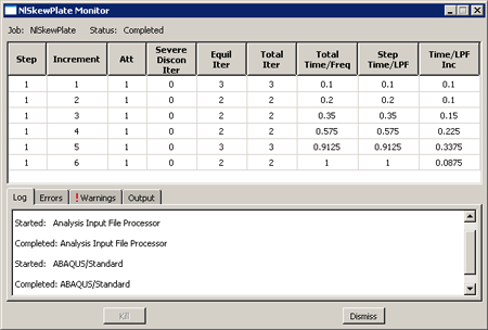
Figure 8–12 shows the contents of the Job Monitor for this nonlinear skewed plate example.
The first column shows the step number—in this case there is only one step. The second column gives the increment number. The sixth column shows the number of iterations ABAQUS/Standard needed to obtain a converged solution in each increment; for example, ABAQUS/Standard needed three iterations in increment 1. The eighth column shows the total step time completed, and the ninth column shows the increment size (This example shows how ABAQUS/Standard automatically controls the increment size and, therefore, the proportion of load applied in each increment. In this analysis ABAQUS/Standard applied 10% of the total load in the first increment: you specified ![]() to be 0.1 and the step time to be 1.0. ABAQUS/Standard needed three iterations to converge to a solution in the first increment. ABAQUS/Standard only needed two iterations in the second increment, so it automatically increased the size of the next increment by 50% to
to be 0.1 and the step time to be 1.0. ABAQUS/Standard needed three iterations to converge to a solution in the first increment. ABAQUS/Standard only needed two iterations in the second increment, so it automatically increased the size of the next increment by 50% to ![]() = 0.15. ABAQUS/Standard also increased
= 0.15. ABAQUS/Standard also increased ![]() in both the fourth and fifth increments. It adjusted the final increment size to be just enough to complete the analysis; in this case the final increment size was 0.0875.
in both the fourth and fifth increments. It adjusted the final increment size to be just enough to complete the analysis; in this case the final increment size was 0.0875.
In addition to allowing you to monitor the progress of your analysis job, ABAQUS/CAE provides a visual diagnostics tool to help you understand the convergence behavior of your job and debug the model if necessary. ABAQUS/Standard stores information in the output database for each step, increment, attempt, and iteration of an analysis. This diagnostic information is saved automatically for every job that you run. If an analysis takes longer than expected or terminates prematurely, you can view the job diagnostic information in ABAQUS/CAE to help determine the cause and to identify ways to correct the model.
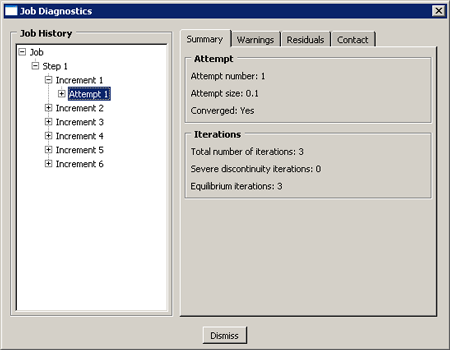
Enter the Visualization module, and open the output database file NlSkewPlate.odb to examine the convergence history. From the main menu bar, select Tools![]() Job Diagnostics to open the Job Diagnostics dialog box. Click the “
Job Diagnostics to open the Job Diagnostics dialog box. Click the “![]() ” symbols in the Job History list to expand the list to include the steps, increments, attempts, and iterations in the analysis job. For example, under Increment 1, select Attempt 1, as shown in Figure 8–13.
” symbols in the Job History list to expand the list to include the steps, increments, attempts, and iterations in the analysis job. For example, under Increment 1, select Attempt 1, as shown in Figure 8–13.
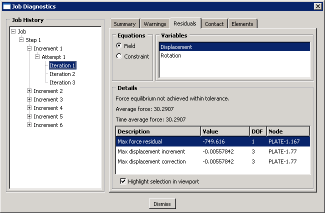
As shown in Figure 8–14, the Residuals tabbed page displays the values of the average force, ![]() , and time average force,
, and time average force, ![]() , in the model.
, in the model.
In this example the initial time increment is 0.1 seconds, as specified in the step definition. The average force for the increment is 30.29 N; and the time average force, ![]() , has the same value since this is the first increment. The largest residual force in the model,
, has the same value since this is the first increment. The largest residual force in the model, ![]() , is –749.6 N, which is clearly greater than 0.005 ×
, is –749.6 N, which is clearly greater than 0.005 × ![]() .
. ![]() occurred at node 167 in degree of freedom 1. ABAQUS/Standard must also check for equilibrium of the moments in the model since this model includes shell elements. The moment/rotation field also failed to satisfy the equilibrium check.
occurred at node 167 in degree of freedom 1. ABAQUS/Standard must also check for equilibrium of the moments in the model since this model includes shell elements. The moment/rotation field also failed to satisfy the equilibrium check.
Although failure to satisfy the equilibrium check is enough to cause ABAQUS/Standard to try another iteration, you should also examine the displacement correction. In the first iteration of the first increment of the first step the largest increment of displacement, ![]() , and the largest correction to displacement,
, and the largest correction to displacement, ![]() , are both –5.578 × 10⁻³ m; and the largest increment of rotation and correction to rotation are both –1.598 × 10⁻² radians. Since the incremental values and the corrections are always equal in the first iteration of the first increment of the first step, the check that the largest corrections to nodal variables are less than 1% of the largest incremental values will always fail. However, if ABAQUS/Standard judges the solution to be linear (a judgement based on the magnitude of the residuals,
, are both –5.578 × 10⁻³ m; and the largest increment of rotation and correction to rotation are both –1.598 × 10⁻² radians. Since the incremental values and the corrections are always equal in the first iteration of the first increment of the first step, the check that the largest corrections to nodal variables are less than 1% of the largest incremental values will always fail. However, if ABAQUS/Standard judges the solution to be linear (a judgement based on the magnitude of the residuals, ![]() < 10–8
< 10–8![]() ), it will ignore this criterion.
), it will ignore this criterion.
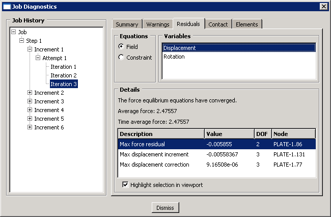
Since ABAQUS/Standard did not find an equilibrium solution in the first iteration, it tries a second iteration. The residual information for the second iteration is shown in Figure 8–15.
In the second iteration ![]() has fallen to –0.173 N at node 167 in degree of freedom 1. However, equilibrium is not satisfied in this iteration because 0.005 ×
has fallen to –0.173 N at node 167 in degree of freedom 1. However, equilibrium is not satisfied in this iteration because 0.005 × ![]() , where
, where ![]() = 2.49 N, is still less than
= 2.49 N, is still less than ![]() . The displacement correction criterion also failed again because
. The displacement correction criterion also failed again because ![]() = –7.055 × 10⁻⁵, which occurred at node 5 in degree of freedom 1, is more than 1% of
= –7.055 × 10⁻⁵, which occurred at node 5 in degree of freedom 1, is more than 1% of ![]() = –5.584 × 10⁻³, the maximum displacement increment.
= –5.584 × 10⁻³, the maximum displacement increment.
Both the moment residual check and the largest correction to rotation check were satisfied in this second iteration; however, ABAQUS/Standard must perform another iteration because the solution did not pass the force residual check (or the largest correction to displacement criterion). The residual information for the additional iteration necessary to obtain a solution in the first increment is shown in Figure 8–16.
After the third iteration ![]() = 2.476 N and
= 2.476 N and ![]() = –5.855 × 10⁻³ N at node 86 in degree of freedom 2. These values satisfy
= –5.855 × 10⁻³ N at node 86 in degree of freedom 2. These values satisfy ![]() < 0.005 ×
< 0.005 × ![]() , so the force residual check is satisfied. Comparing
, so the force residual check is satisfied. Comparing ![]() to the largest increment of displacement shows that the displacement correction is below the required tolerance. The solution for the forces and displacements has, therefore, converged. The checks for both the moment residual and the rotation correction continue to be satisfied, as they have been since the second iteration. With a solution that satisfies equilibrium for all variables (displacement and rotation in this case), the first load increment is complete. The attempt summary (Figure 8–13) shows the number of iterations that were required for this increment and the size of the increment.
to the largest increment of displacement shows that the displacement correction is below the required tolerance. The solution for the forces and displacements has, therefore, converged. The checks for both the moment residual and the rotation correction continue to be satisfied, as they have been since the second iteration. With a solution that satisfies equilibrium for all variables (displacement and rotation in this case), the first load increment is complete. The attempt summary (Figure 8–13) shows the number of iterations that were required for this increment and the size of the increment.
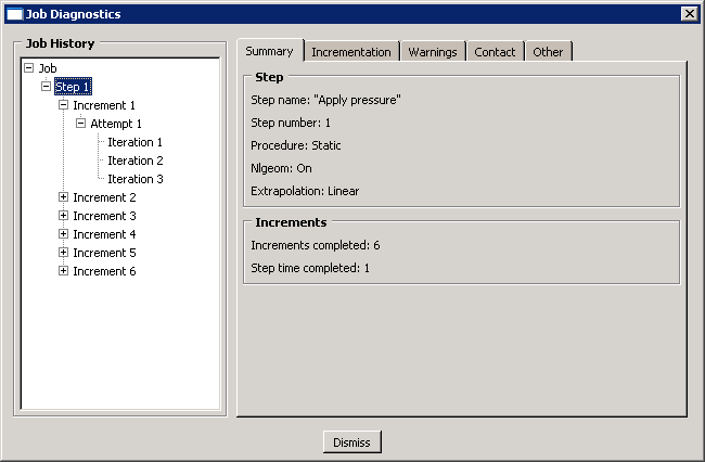
ABAQUS/Standard continues this process of applying an increment of load then iterating to find a solution until it completes the whole analysis (or reaches the maximum increment that you specified). In this analysis it required five more increments. The step summary is shown in Figure 8–17.
In addition to the residual information discussed above, analysis warning messages related to numerical singularities, zero pivots, and negative eigenvalues, if they exist, are displayed in the Job Diagnostics dialog box (in the Warnings tabbed page). Always investigate the cause of these warnings.
You will now postprocess the results.
Showing the available frames
To begin this exercise, determine the available output frames (the increment intervals at which results were written to the output database).
To show the available frames:
From the main menu bar, select Result![]() Step/Frame.
Step/Frame.
The Step/Frame dialog box appears.
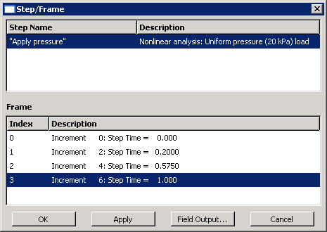
During the analysis ABAQUS/Standard wrote field output results to the output database file every second increment, as was requested. ABAQUS/CAE displays the list of the available frames, as shown in Figure 8–18.
The list tabulates the steps and increments for which field variables are stored. This analysis consisted of a single step with six increments. The results for increment 0 (the initial state of the step) are saved by default, and you saved data for increments 2, 4, and 6. By default, ABAQUS/CAE always uses the data for the last available increment saved in the output database file.
Click OK to dismiss the Step/Frame dialog box.
Displaying the deformed and undeformed model shapes
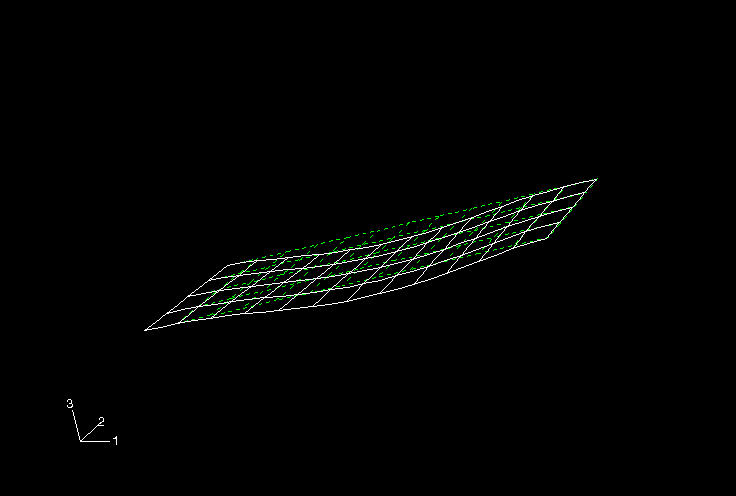
Use the Allow Multiple Plot States ![]() tool to display the deformed model shape with the undeformed model shape superimposed. Set the render style for both images to wireframe, and toggle off the translucency of the superimposed plot. Rotate the view to obtain a plot similar to that shown in Figure 8–19. (For clarity, the edges of the undeformed shape are plotted using a dashed style.)
tool to display the deformed model shape with the undeformed model shape superimposed. Set the render style for both images to wireframe, and toggle off the translucency of the superimposed plot. Rotate the view to obtain a plot similar to that shown in Figure 8–19. (For clarity, the edges of the undeformed shape are plotted using a dashed style.)
Using results from other frames
You can evaluate the results from other increments saved to the output database file by selecting the appropriate frame.
To select a new frame:
From the main menu bar, select Result![]() Step/Frame.
Step/Frame.
The Step/Frame dialog box appears.
Select Increment 4 from the Frame menu.
Click OK to apply your changes and to close the Step/Frame dialog box.
Any plots now requested will use results from increment 4. Repeat this procedure, substituting the increment number of interest, to move through the output database file.
Note: Alternatively, you may use the Frame Selector dialog box to select a results frame.
X–Y plotting
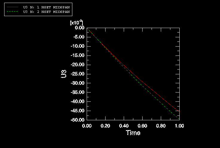
You saved the displacements of the midspan nodes (node set Midspan) in the history portion of the output database file NlSkewPlate.odb for each increment of the simulation. You can use these results to create X–Y plots. In particular, you will plot the vertical displacement history of the nodes located at the edges of the plate midspan.
To create X–Y plots of the midspan displacements:
First, display only the nodes in the node set named Midspan: in the Results Tree, expand the Node Sets container underneath the output database file named NlSkewPlate.odb. Click mouse button 3 on the set named MIDSPAN, and select Replace from the menu that appears.
Use the Common Plot Options dialog box to show the node labels (i.e., numbers) to determine which nodes are located at the edges of the plate midspan.
In the Results Tree, expand the History Output container. Locate the output labeled as follows: Spatial displacement: U3 at Node xxx in NSET MIDSPAN. Each of these curves represents the vertical motion of one of the midspan nodes.
Select (using [Ctrl]+Click) the vertical motion of the two midspan edge nodes. Use the node labels to determine which curves you need to select.
Click mouse button 3, and select Plot from the menu that appears.
ABAQUS reads the data for both curves from the output database file and plots a graph similar to the one shown in Figure 8–20. (For clarity, the second curve has been changed to a dashed line.)
The nonlinear nature of this simulation is clearly seen in these curves: as the analysis progresses, the plate stiffens. The effects of geometric nonlinearity mean that a structure's stiffness changes as it deforms. In this simulation the plate gets stiffer as it deforms due to membrane effects. Therefore, the resulting peak displacement is less than that predicted by the linear analysis, which did not include this effect.
You can create X–Y curves from either history or field data stored in the output database (.odb) file. X–Y curves can also be read from an external file or they can be typed into the Visualization module interactively. Once curves have been created, their data can be further manipulated and plotted to the screen in graphical form.
The X–Y plotting capability of the Visualization module is discussed further in Chapter 10, “Materials.”
Tabular data
Create a tabular data report of the midspan displacements. Use the node set Midspan to create the appropriate display group and the frame selector to choose the final frame. The contents of the report are shown below.
Field Output Report

Source 1
---------

   ODB: NlSkewPlate.odb
   Step: Apply pressure
   Frame: Increment      6: Step Time =    1.000

Loc 1 : Nodal values from source 1

Output sorted by column "Node Label".

Field Output reported at nodes for part: PLATE-1


            Node            U.U1            U.U2            U.U3
           Label          @Loc 1          @Loc 1          @Loc 1
-----------------------------------------------------------------
               1    -2.68697E-03    -747.394E-06    -49.4696E-03
               2    -2.27869E-03    -806.331E-06    -45.4817E-03
               7    -2.57405E-03    -759.298E-06    -48.5985E-03
               8    -2.49085E-03    -775.165E-06    -47.7038E-03
               9     -2.4038E-03    -793.355E-06     -46.533E-03
              66    -2.62603E-03    -750.246E-06    -49.0086E-03
              70    -2.53886E-03    -762.497E-06    -48.1876E-03
              73    -2.45757E-03    -778.207E-06     -47.144E-03
              76    -2.36229E-03    -794.069E-06    -45.9613E-03


  Minimum           -2.68697E-03    -806.331E-06    -49.4696E-03

         At Node               1               2               1
  Maximum           -2.27869E-03    -747.394E-06    -45.4817E-03

         At Node               2               1               2
Compare these with the displacements from the linear analysis in Chapter 5, “Using Shell Elements.” The maximum displacement at the midspan in this simulation is about 9% less than that predicted from the linear analysis. Including the nonlinear geometric effects in the simulation reduces the vertical deflection (U3) of the midspan of the plate.
Another difference between the two analyses is that in the nonlinear simulation there are nonzero deflections in the 1- and 2-directions. What effects make the in-plane displacements, U1 and U2, nonzero in the nonlinear analysis? Why is the vertical deflection of the plate less in the nonlinear analysis?
The plate deforms into a curved shape: a geometry change that is taken into account in the nonlinear simulation. As a consequence, membrane effects cause some of the load to be carried by membrane action rather than by bending alone. This makes the plate stiffer. In addition, the pressure loading, which is always normal to the plate's surface, starts to have a component in the 1- and 2-directions as the plate deforms. The nonlinear analysis includes the effects of this stiffening and the changing direction of the pressure. Neither of these effects is included in the linear simulation.
The differences between the linear and nonlinear simulations are sufficiently large to indicate that a linear simulation is not adequate for this plate under this particular loading condition.
For five-degree-of-freedom shells, such as the S8R5 element used in this analysis, ABAQUS/Standard does not output total rotations at the nodes.
As an optional exercise, you can modify the model and run a dynamic analysis of the skew plate in ABAQUS/Explicit. To do so, you must add a density of 7800 kg/m3 to the material definition for steel, replace the existing step with an explicit dynamic step, and change the element library to Explicit. In addition, you should edit the history output requests to write the translations and rotations for the set MidSpan to the output database file. This information will be helpful in evaluating the dynamic response of the plate. After making the appropriate model changes, you can create and run a new job to examine the transient dynamic effects in the plate under a suddenly applied load.