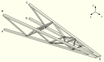
A light-service, cargo crane is shown in Figure 6–10. You have been asked to determine the static deflections of the crane when it carries a load of 10 kN. You should also identify the critical members and joints in the structure: i.e., those with the highest stresses and loads. Because this is a static analysis you will analyze the cargo crane using ABAQUS/Standard.
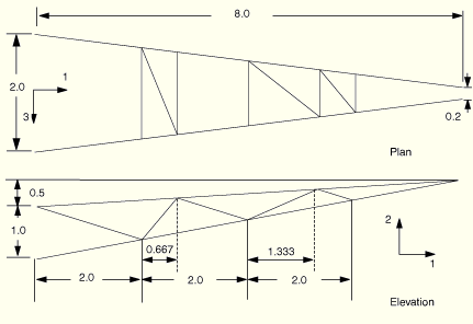
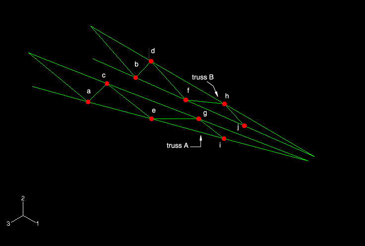
The crane consists of two truss structures joined together by cross bracing. The two main members in each truss structure are steel box beams (box cross-sections). Each truss structure is stiffened by internal bracing, which is welded to the main members. The cross bracing connecting the two truss structures is bolted to the truss structures. These connections can transmit little, if any, moment and, therefore, are treated as pinned joints. Both the internal bracing and cross bracing use steel box beams with smaller cross-sections than the main members of the truss structures. The two truss structures are connected at their ends (at point E) in such a way that allows independent movement in the 3-direction and all of the rotations, while constraining the displacements in the 1- and 2-directions to be the same. The crane is welded firmly to a massive structure at points A, B, C, and D. The dimensions of the crane are shown in Figure 6–11. In the following figures, truss A is the structure consisting of members AE, BE, and their internal bracing; and truss B consists of members CE, DE, and their internal bracing.
The ratio of the typical cross-section dimension to global axial length in the main members of the crane is much less than 1/15. The ratio is approximately 1/15 in the shortest member used for internal bracing. Therefore, it is valid to use beam elements to model the crane.
We will now discuss how to create this model using ABAQUS/CAE. A Python script is provided in “Cargo crane,” Section A.4. When this script is run through ABAQUS/CAE, it creates the complete analysis model for this problem. Run this script if you encounter difficulties following the instructions given below or if you wish to check your work. Instructions on how to fetch and run the script are given in Appendix A, “Example Files.”
If you do not have access to ABAQUS/CAE or another preprocessor, the input file required for this problem can be created manually, as discussed in “Example: cargo crane,” Section 6.4 of Getting Started with ABAQUS/Standard: Keywords Version.
Creating the parts
The welded joints between the internal bracing and main members in the crane provide complete continuity of the translations and rotations from one region of the model to the next. Therefore, you need only a single geometric entity (i.e., vertex) at each welded joint in the model. A single part is used to represent the internal bracing and main members. For convenience, both truss structures will be treated as a single part.
The bolted joints, which connect the cross bracing to the truss structures, and the connection at the tip of the truss structures are different from the welded joint connections. Since these joints do not provide complete continuity for all degrees of freedom, separate vertices are needed for connection. Thus, the cross bracing must be treated as a separate part since distinct geometric entities are required to model the bolted joints. Appropriate constraints between the separate vertices must be specified.
We begin by discussing a technique to define the truss geometry. Since the two truss structures are identical, it is sufficient to define the base feature of the part using only the geometry of a single truss structure. The sketch of the truss geometry can be saved and then used to add the second truss structure to the part definition.
The dimensions shown in Figure 6–11 are relative to a global Cartesian coordinate system. The base feature, however, must be sketched in a local plane. To make the sketching easier, datum features will be used. A datum plane, parallel to one of the trusses (truss B in Figure 6–10, for example), will serve as the sketch plane. The orientation of the sketch plane will be defined using a datum axis.
To define the geometry of a single truss:
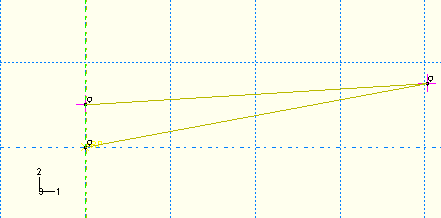
To create a datum plane, a part must first be created. A part consisting of a single reference point will serve this purpose. Begin by creating a three-dimensional, deformable, point part. Set the approximate part size to 20.0, and name the part Truss. Place the point at the origin. This point represents point D in Figure 6–10.
Using the Create Datum Point: Offset From Point tool ![]() , create two datum points at distances of (0, 1, 0) and (8, 1.5, 0.9) from the reference point. These points represent points C and E, respectively, in Figure 6–10. Reset the view using the Auto-Fit View tool in the toolbar to see the full model.
, create two datum points at distances of (0, 1, 0) and (8, 1.5, 0.9) from the reference point. These points represent points C and E, respectively, in Figure 6–10. Reset the view using the Auto-Fit View tool in the toolbar to see the full model.
Using the Create Datum Plane: 3 Points tool ![]() , create a datum plane to serve as the sketch plane. Select the reference point first, and then select the other two datum points in a counterclockwise fashion.
, create a datum plane to serve as the sketch plane. Select the reference point first, and then select the other two datum points in a counterclockwise fashion.
Note: While selecting the points in this way is not required, it will make certain operations that follow easier. For example, by selecting the points in a counterclockwise order, the normal to the plane points out of the viewport and the sketch plane will be oriented automatically in the 1–2 view in the Sketcher. If you select the points in a clockwise order, the plane's normal will point into the viewport and the sketch plane will have to be adjusted in the Sketcher.
Using the Create Datum Axis: Principal Axis tool ![]() , create a datum axis parallel to the Y-Axis. As noted earlier, this axis will be used to position the sketch plane.
, create a datum axis parallel to the Y-Axis. As noted earlier, this axis will be used to position the sketch plane.
You are now ready to sketch the geometry. Use the Create Wire: Planar tool ![]() to enter the Sketcher. Select the datum plane as the plane on which to sketch the wire geometry; select the datum axis as the axis that will appear vertical and to the left of the sketch. You may need to resize your view to select these entities.
to enter the Sketcher. Select the datum plane as the plane on which to sketch the wire geometry; select the datum axis as the axis that will appear vertical and to the left of the sketch. You may need to resize your view to select these entities.
Once in the Sketcher, use the Sketcher Options tool to change the Sheet size to 20 and the Grid spacing to 2. Zoom in to see the datum points more clearly.
Note: If the sketch plane is not oriented in the 1–2 plane, use the Views Toolbox to change to the 1–2 view.
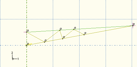
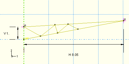
Next, create a series of connected lines as shown in Figure 6–13 to approximate the interior bracing of the truss.
At this stage, the layout of the interior bracing is arbitrary and is intended only as a rough approximation of the true shape. The endpoints of the lines, however, must snap to the edges of the main truss members. This is indicated in the figure by the presence of small circles next to the intersections of the interior bracing with the main members. Avoid creating 90° angles because that will introduce unwanted additional constraints.Split the edges of the main members at the points where they intersect the interior bracing.
Dimension the vertical distance between the left endpoints of the sketch and the horizontal distance between the reference point and the right endpoint of the sketch, as shown in Figure 6–14. These dimensions will act as additional constraints on the sketch. Accept the values shown in the prompt area when creating the dimensions. These values represent the dimensions of the part, projected from the global Cartesian coordinate system (depicted in Figure 6–11) to the local sketch plane.
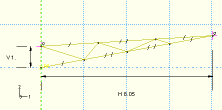
To complete the sketch, recognize from Figure 6–11 that the interior bracing breaks the main members into equal length segments on both its top and bottom edges. Thus, impose equal length constraints on the segments of the top edge of the main member; repeat this operation for the bottom edge of the main member. The final sketch appears as shown in Figure 6–15.
Using the Save Sketch As tool ![]() , save the sketch as Truss.
, save the sketch as Truss.
Click Done to exit the Sketcher and to save the base feature of the part.
The other truss will also be added as a planar wire feature by projecting the truss created here onto a new datum plane.
To define the geometry of the second truss structure:
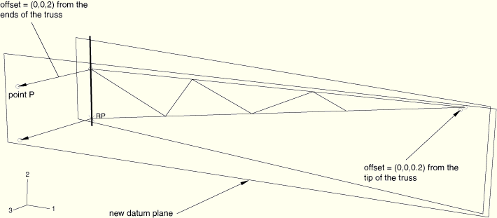
Define three datum points using offsets from the end points of the truss, as shown in Figure 6–16. The offsets from the parent vertices are indicated in the figure. You may need to rotate your sketch to see the datum points.
Create a datum plane using these three points. As before, the points defining the plane should be chosen in a counterclockwise order.
Use the Create Wire: Planar tool to add a feature to the part. Select the new datum plane as the sketch plane and the datum axis created earlier as the edge that will appear vertical and on the left of the sketch.
Note: If the sketch plane is not oriented in the 1–2 plane, use the Views Toolbox to change to the 1–2 view.
Use the Add Sketch tool ![]() to retrieve the truss sketch. Translate the sketch by selecting the vertex at the top left end of the new truss as the starting point of the translation vector and the datum point labeled P in Figure 6–16 as the endpoint of the vector. Zoom in and rotate the view as necessary to facilitate your selections.
to retrieve the truss sketch. Translate the sketch by selecting the vertex at the top left end of the new truss as the starting point of the translation vector and the datum point labeled P in Figure 6–16 as the endpoint of the vector. Zoom in and rotate the view as necessary to facilitate your selections.
Note: If the points defining either the original or new datum plane were not selected in a counterclockwise order, you will have to mirror the sketch before translating it. If necessary, cancel the sketch retrieval operation, create the necessary construction line for mirroring, and retrieve the sketch again.
Click Done in the prompt area to exit the Sketcher.
The final truss part is shown in Figure 6–17. The visibility of all datum and reference geometry has been suppressed.
Figure 6–17 Final geometry of the truss structures; highlighted vertices indicate the locations of the pin joints.
Recall that the cross bracing must be treated as a separate part to properly represent the pin joints between it and the trusses. The easiest way to sketch the cross bracing, however, is to create wire features directly between the locations of the joints in the trusses. Thus, we will adopt the following method to create the cross bracing part: first, a copy of the truss part will be created and the wires representing the cross brace will be added to it (we cannot use this new part as is because the vertices at the joints are shared and, thus, cannot represent a pin joint); then, we will use the cut feature available in the Assembly module to perform a Boolean cut between the truss with the cross brace and the truss without the cross brace, leaving the cross brace geometry as a distinct part. The procedure is described in detail below.
To create the cross brace geometry:
In the Model Tree, click mouse button 3 on the Truss item underneath the Parts container and select Copy from the menu that appears. In the Part Copy dialog box, name the new part Truss-all, and click OK.
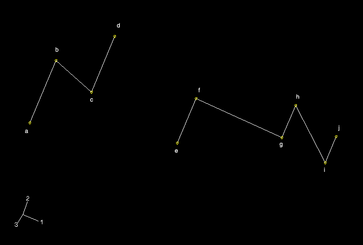
The pin locations are highlighted in Figure 6–17. Use the Create Wire: Point to Point tool. In the Edit Wires dialog box, toggle on Chained wires and click Add to add the cross bracing geometry to the new part, as shown in Figure 6–18 (the vertices in this figure correspond to those labeled in Figure 6–17; the visibility of the truss in Figure 6–18 has been suppressed). Use the following coordinates to specify a similar view: Viewpoint (1.19, 5.18, 7.89), Up vector (–0.40, 0.76, –0.51).
Tip:
If you make a mistake while connecting the cross bracing geometry, you can delete a line using the Delete Feature tool ![]() ; you cannot recover deleted features.
; you cannot recover deleted features.
Create an instance of each part (Truss and Truss-all).
From the main menu bar of the Assembly module, select Instance![]() Merge/Cut. In the Merge/Cut Instances dialog box, name the new part Cross brace, select Cut geometry in the Operations field, and click Continue.
Merge/Cut. In the Merge/Cut Instances dialog box, name the new part Cross brace, select Cut geometry in the Operations field, and click Continue.
From the Instance List, select Truss-all-1 as the instance to be cut and Truss-1 as the instance that will make the cut.
After the cut is made, a new part named Cross brace is created that contains only the cross brace geometry. The current model assembly contains only an instance of this part; the original part instances are suppressed by default. Since we will need to use the original truss in the model assembly, click mouse button 3 on Truss-1 underneath the Instances container and select Resume from the menu that appears to resume this part instance.
We now define the beam section properties.
Defining beam section properties
Since the material behavior in this simulation is assumed to be linear elastic, it is more efficient from a computational point of view to precompute the beam section properties. Assume the trusses and bracing are made of a mild strength steel with ![]() = 200.0 × 10⁹ Pa,
= 200.0 × 10⁹ Pa, ![]() = 0.25, and
= 0.25, and ![]() = 80.0 × 10⁹ Pa. All the beams in this structure have a box-shaped cross-section.
= 80.0 × 10⁹ Pa. All the beams in this structure have a box-shaped cross-section.
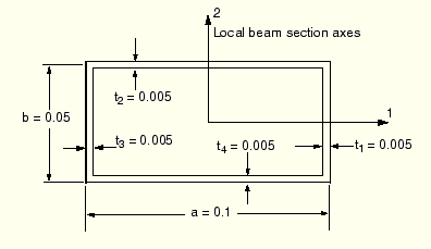
A box-section is shown in Figure 6–19. The dimensions shown in Figure 6–19 are for the main members of the two trusses in the crane.
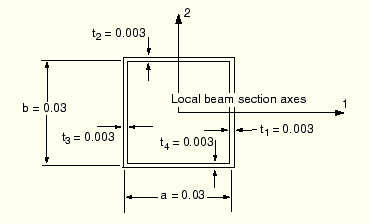
The dimensions of the beam sections for the bracing members are shown in Figure 6–20.To define the beam section properties:
In the Model Tree, double-click the Profiles container to create a box profile for the main members of the truss structures; then, create a second profile for the internal and cross bracing. Name the profiles MainBoxProfile and BraceBoxProfile, respectively. Use the dimensions shown in Figure 6–19 and Figure 6–20 to complete the profile definitions.
Create one Beam section for the main members of the truss structures and one for the internal and cross bracing. Name the sections MainMemberSection and BracingSection, respectively.
For both section definitions, specify that section integration will be performed before the analysis. When this type of section integration is chosen, material properties are defined as part of the section definition rather than in a separate material definition.
Choose MainBoxProfile for the main members' section definition, and BraceBoxProfile for the bracing section definition.
Click the Basic tab, and enter the Young's and shear moduli noted earlier in the appropriate fields of the data table.
Enter the Section Poisson's ratio in the appropriate text field of the Edit Beam Section dialog box.
Assign MainMemberSection to the geometry regions representing the main members of the trusses and BracingSection to the regions representing the internal and cross bracing members. Use the Part list located below the toolbar to retrieve each part. You can ignore the Truss-all part since it is no longer needed.
Defining beam section orientations
The beam section axes for the main members should be oriented such that the beam 1-axis is orthogonal to the plane of the truss structures shown in the elevation view (Figure 6–11) and the beam 2-axis is orthogonal to the elements in that plane. The approximate ![]() -vector for the internal truss bracing is the same as for the main members of the respective truss structures.
-vector for the internal truss bracing is the same as for the main members of the respective truss structures.
In its local coordinate system, the Truss part is oriented as shown in Figure 6–21.
From the main menu bar of the Property module, select AssignFrom the main menu bar, select Assign![]() Tangent to specify the beam tangent directions. Flip the tangent directions as necessary so that they appear as shown in Figure 6–22.
Tangent to specify the beam tangent directions. Flip the tangent directions as necessary so that they appear as shown in Figure 6–22.
While both the cross bracing and the bracing within each truss structure have the same beam section geometry, they do not share the same orientation of the beam section axes. Since the square cross bracing members are subjected to primarily axial loading, their deformation is not sensitive to cross-section orientation; thus, we make some assumptions so that the orientation of the cross-bracing is somewhat easier to specify. All of the beam normals (![]() -vectors) should lie approximately in the plane of the plan view of the cargo crane (see Figure 6–20). This plane is skewed slightly from the global 1–3 plane. A simple method for defining such an orientation is to provide an approximate
-vectors) should lie approximately in the plane of the plan view of the cargo crane (see Figure 6–20). This plane is skewed slightly from the global 1–3 plane. A simple method for defining such an orientation is to provide an approximate ![]() -vector that is orthogonal to this plane. The vector should be nearly parallel to the global 2-direction. Therefore, specify
-vector that is orthogonal to this plane. The vector should be nearly parallel to the global 2-direction. Therefore, specify ![]() = (0.0, 1.0, 0.0) for the cross bracing so that it is aligned with the part (and as we shall see later, global) y-axis.
= (0.0, 1.0, 0.0) for the cross bracing so that it is aligned with the part (and as we shall see later, global) y-axis.
Beam normals
In this model you will have a modeling error if you provide data that only define the orientation of the approximate ![]() -vector. Unless overridden, the averaging of beam normals (see “Beam element curvature,” Section 6.1.3) causes ABAQUS to use incorrect geometry for the cargo crane model. To see this, you can use the Visualization module to display the beam section axes and beam tangent vectors (see “Postprocessing,” Section 6.4.2). Without any further modification to the beam normal directions, the normals in the crane model would appear to be correct in the Visualization module; yet, they would be, in fact, slightly incorrect.
-vector. Unless overridden, the averaging of beam normals (see “Beam element curvature,” Section 6.1.3) causes ABAQUS to use incorrect geometry for the cargo crane model. To see this, you can use the Visualization module to display the beam section axes and beam tangent vectors (see “Postprocessing,” Section 6.4.2). Without any further modification to the beam normal directions, the normals in the crane model would appear to be correct in the Visualization module; yet, they would be, in fact, slightly incorrect.
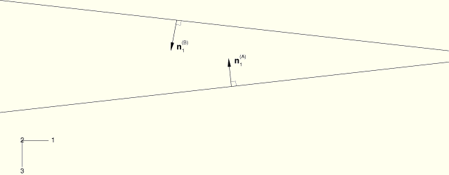
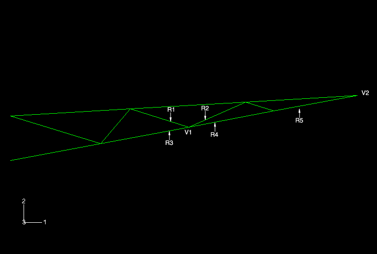
Figure 6–23 shows the geometry of the truss structure.
Referring to this figure, the correct geometry for the crane model requires three independent beam normals at vertex V1: one each for regions R1 and R2 and a single normal for regions R3 and R4. Using the ABAQUS logic for averaging normals, it becomes readily apparent that the beam normal at vertex V1 in region R2 would be averaged with the normals at this point for the adjacent regions. In this case the important part of the averaging logic is that normals that subtend an angle less than 20° with the reference normal are averaged with the reference normal to define a new reference normal. Assume the original reference normal at this point is the normal for regions R3 and R4. Since the normal at vertex V1 in region R2 subtends an angle less than 20° with the original reference normal, it is averaged with the original normal to define a new reference normal at that location. On the other hand, since the normal at vertex V1 in region R1 subtends an angle of approximately 30° with the original reference normal, it will have an independent normal.This incorrect average normal means that the elements that will be created on regions R2, R3, and R4 and that share the node created at vertex V1 would have a section geometry that twists about the beam axis from one end of the element to the other, which is not the intended geometry. You should specify the normal directions explicitly at positions where the subtended angle between adjacent regions will be less than 20°. This will prevent ABAQUS from applying its averaging algorithm. In this problem you must do this for the corresponding regions on both sides of the crane.
There is also a problem with the normals at vertex V2 at the tip of the truss structure, again because the angle between the two regions attached to this vertex is less than 20°. Since we are modeling straight beams, the normals are constant at both ends of each beam. This can be corrected by explicitly specifying the beam normal direction. As before, you must do this for the corresponding regions on both sides of the crane.
Currently, the only way to specify beam normal directions in ABAQUS/CAE is with the Keywords Editor. The Keywords Editor is a specialized text editor that allows you to modify the ABAQUS input file generated by ABAQUS/CAE before submitting it for analysis. Thus, it allows you to add ABAQUS/Standard or ABAQUS/Explicit functionality when such functionality is not supported by the current version of ABAQUS/CAE. For more information on the Keywords Editor, see “Adding unsupported keywords to your ABAQUS/CAE model,” Section 9.9.1 of the ABAQUS/CAE User's Manual.
You will specify the beam normal directions later.
Creating an assembly
We now focus on assembling the model. Since the parts are already aligned with the global Cartesian coordinate system shown in Figure 6–11, no further manipulations of the parts are necessary.
At this point, however, it is convenient to define assembly-level geometry sets that will be used later. In the Model Tree, double-click the Assembly container. Define a geometry set containing the vertices corresponding to points A through D (refer to Figure 6–10 for the exact locations), and name the set Attach. When defining this set, be sure to select the vertices of the truss and not reference points. You may need to use the Selection Options tool ![]() to aid in your selection.
to aid in your selection.
In addition, create sets at the vertices located at the tips of the trusses (location E in Figure 6–10). Name the sets Tip-a and Tip-b, with Tip-a being the geometry set associated with truss A (see Figure 6–17). Finally, create a set for each region where beam normals will be specified, referring to Figure 6–17 and Figure 6–23. For truss A, create a set named Inner-a for the region indicated by R2 and a set named Leg-a for the region indicated by R5; create corresponding sets Inner-b and Leg-b for truss B.
Creating a step definition and specifying output
Create a single static, general step. Name the step Tip load, and enter the following step description: Static tip load on crane.
Write the displacements (U) and reaction forces (RF) at the nodes and the section forces (SF) in the elements to the output database as field output for postprocessing with ABAQUS/CAE.
Defining constraint equations
Constraints between nodal degrees of freedom are specified in the Interaction module. The form of each equation is
![]()
In the crane model the tips of the two trusses are connected together such that degrees of freedom 1 and 2 (the translations in the 1- and 2-directions) are equal, while the other degrees of freedom (3–6) are independent. We need two linear constraints, one equating degree of freedom 1 at the two vertices and the other equating degree of freedom 2.
To create linear equations:
In the Model Tree, double-click the Constraints container. Name the constraint TipConstraint-1, and specify an equation constraint.
In the Edit Constraint dialog box, enter a coefficient of 1.0, the set name Tip-a, and degree of freedom 1 in the first row. In the second row, enter a coefficient of -1.0, the set name Tip-b, and degree of freedom 1. Click OK.
This defines the constraint equation for degree of freedom 1.
Note: Text input is case-sensitive in ABAQUS/CAE.
Click mouse button 3 on the TipConstraint-1 item underneath the Constraints container, and select Copy from the menu that appears. Copy TipConstraint-1 to TipConstraint-2.
Double-click TipConstraint-2 underneath the Constraints container to edit it. Change the degree of freedom on both lines to 2.
The degrees of freedom associated with the first set defined in an equation are eliminated from the stiffness matrix. Therefore, this set should not appear in other constraint equations, and boundary conditions should not be applied to the eliminated degrees of freedom.
Modeling the pin joint between the cross bracing and the trusses
The cross bracing, unlike the internal truss bracing, is bolted to the truss members. You can assume that these bolted connections are unable to transmit rotations or torsion. The duplicate vertices that were defined at these locations are needed to define this constraint. In ABAQUS such constraints can be defined using multi-point constraints, constraint equations, or connectors. In this example the last approach is adopted.
Connectors allow you to model a connection between any two points in a model assembly (or between any single point in the assembly and the ground). A large library of connectors is available in ABAQUS. See “Connector element library,” Section 25.1.4 of the ABAQUS Analysis User's Manual, for a complete list and a description of each connector type.
The JOIN connector will be used to model the bolted connection. The pinned joint created by this connector constrains the displacements to be equal but the rotations (if they exist) remain independent.
In ABAQUS/CAE connectors are modeled using connector section assignments. You create an assembly-level wire feature to define the connector geometry and a connector section to define the connection type. You can model connectors at all of the pin joints using one connector section assignment. You create the connector section assignment by selecting multiple wires and specifying a connector section to assign to the selected wires (similar to the association between elements and their section properties). Thus, the wire feature will be defined first, followed by the connector section and the connector section assignment.
To define an assembly-level wire feature:
From the main menu bar in the Interaction module, select Connector![]() Geometry
Geometry![]() Point-to-Point Wire. In the Create Wires dialog box, accept the default Disjoint wires option to select points that are not automatically connected end-to-end, and click Add.
Point-to-Point Wire. In the Create Wires dialog box, accept the default Disjoint wires option to select points that are not automatically connected end-to-end, and click Add.
In the viewport, double-click each pin joint location (actually, you are picking the same point twice). These are labeled a–j in Figure 6–17. For each joint, this action selects the coincident points in sequence and defines a zero-length wire between the points. Once you have double-clicked each pin joint, click Done in the prompt area.
In the Create Wires dialog box, toggle on Create set of wires. This will facilitate the connector section assignment that follows. Click OK.
To define a connector section:
In the Model Tree, double-click the Connector Sections container. In the Create Connector Section dialog box, select Basic types as the Connection Type. From the list of available translational types, select Join. Accept all other defaults, and click Continue.
No additional section specifications are required. Thus, in the connector section editor that appears, click OK.
To define a connector section assignment:
In the Model Tree, double-click the Connector Assignments container. Click Sets on the right side of the prompt area, select Wire-1–Set-1 from the Region Selection dialog box that appears. If you had not created a set when you created the wire feature, you could use drag-select to select the zero-length wires in the viewport. Click Continue.
In the connector section assignment editor that appears, accept the default selection for the Section. No orientation specifications are required. Click OK to complete the connector section assignment. Symbols appear in the viewport indicating the presence of the connector section assignment.
Defining loads and boundary conditions
A total load of 10 kN is applied in the negative y-direction to the ends of the truss. Recall there is a constraint equation connecting the y-displacement of sets Tip-a and Tip-b, where the degree of freedom for set Tip-a is eliminated from the system equations. Thus, apply the load as a concentrated force of magnitude 10000 to set Tip-b. Name the load Tip load. Because of the constraint, the load will be carried equally by both trusses.
The crane is attached firmly to the parent structure. Create an encastre boundary condition named Fixed end, and apply it to set Attach.
Creating the mesh
The cargo crane will be modeled with three-dimensional, slender, cubic beam elements (B33). The cubic interpolation in these elements allows us to use a single element for each member and still obtain accurate results under the applied bending load. The mesh that you should use in this simulation is shown in Figure 6–24.
In the Model Tree, expand the Truss item underneath the Parts container. Then double-click Mesh in the list that appears. Specify a global part seed of 2.0 for all regions. Repeat this for the part named Cross brace.
Tip: In the context bar of the Mesh module, select the appropriate part from the Object pull-down list to switch between the parts more readily.
Using the Keywords Editor and defining the job
You will now add the keyword options that are necessary to complete the model definition (namely, the option to define beam normal directions) using the Keywords Editor. Refer to the ABAQUS Keywords Manual for a description of the required syntax, if necessary.
To add options in the Keywords Editor:
In the Model Tree, click mouse button 3 on Model-1 and select Edit Keywords from the menu that appears.
The Edit Keywords dialog box appears containing the input file that has been generated for your model.
In the Keywords Editor each keyword is displayed in its own block. Only text blocks with a white background can be edited. Select the text block that appears just prior to the *END ASSEMBLY option. Click Add After to add an empty block of text.
In the block of text that appears, enter the following:
*NORMAL, TYPE=ELEMENT
Inner-a,  Inner-a, -0.3986,  0.9114,  0.1025
Inner-b,  Inner-b,  0.3986, -0.9114,  0.1025
Leg-a,    Leg-a,   -0.1820,  0.9829,  0.0205
Leg-b,    Leg-b,    0.1820, -0.9829,  0.0205
Tip: Copy and paste data from one location in a text block to another.
When you have finished, click OK to exit the Keywords Editor.
Before continuing, rename the model to Static. This model will later form the basis of the model used in the crane example discussed in Chapter 7, “Linear Dynamics.”
Save your model in a model database file named Crane.cae, and create a job named Crane.
Submit the job for analysis, and monitor the solution progress. If any modeling errors are encountered, correct them; investigate the cause of any warning messages, taking appropriate action as necessary.
Switch to the Visualization module, and open the file Crane.odb. ABAQUS displays an undeformed shape plot of the crane model.
Plotting the deformed model shape
To begin this exercise, plot the deformed model shape with the undeformed model shape superimposed on it. Specify a nondefault view using (0, 0, 1) as the X-, Y-, and Z-coordinates of the viewpoint vector and (0, 1, 0) as the X-, Y-, and Z-coordinates of the up vector.
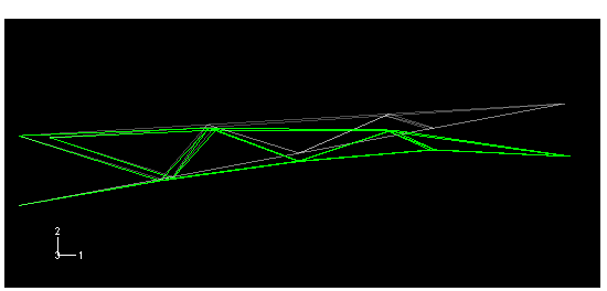
The undeformed shape of the crane superimposed upon the deformed shape is shown in Figure 6–25.
Using display groups to plot element and node sets
You can use display groups to plot existing node and element sets; you can also create display groups by selecting nodes or elements directly from the viewport. You will create a display group containing only the elements associated with the main members in truss structure A.
To create and plot a display group:
In the Results Tree, expand the Sections container underneath the output database file named Crane.odb.
To facilitate your selection change the view back to the default isometric view using the ![]() tool in the toolbar.
tool in the toolbar.
In succession, click the items in the container until the elements associated with the main members in truss A are highlighted in the viewport. Click mouse button 3 on this item and select Replace from the menu that appears.
ABAQUS/CAE now displays only this group of elements.
To save this group, double-click Display Groups in the Results Tree; or use the ![]() tool in the toolbar.
tool in the toolbar.
The Create Display Group dialog box appears.
In the Create Display Group dialog box, click Save As and enter MainA as the name for your display group.
Click Dismiss to close the Create Display Group dialog box.
This display group now appears underneath the Display Groups container in the Results Tree.
Beam cross-section orientation
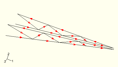
You will now plot the section axes and beam tangents on the undeformed model shape.
To plot the beam section axes:
From the main menu bar, select Plot![]() Undeformed Shape; or use the
Undeformed Shape; or use the ![]() tool in the toolbox to display only the undeformed model shape.
tool in the toolbox to display only the undeformed model shape.
From the main menu bar, select Options![]() Common; then, click the Normals tab in the dialog box that appears.
Common; then, click the Normals tab in the dialog box that appears.
Toggle on Show normals, and accept the default setting of On elements.
In the Style area at the bottom of the Normals page, specify the Length to be Long.
Click OK.
The section axes and beam tangents are displayed on the undeformed shape.
Creating a hard copy
You can save the image of the beam normals to a file for hardcopy output.
To create a PostScript file of the beam normals image:
From the main menu bar, select File![]() Print.
Print.
The Print dialog box appears.
From the Settings area in the Print dialog box, select Black&White as the Rendition type; and toggle on File as the Destination.
Select PS as the Format, and enter beamsectaxes.ps as the File name.
Click PS Options.
The PostScript Options dialog box appears.
From the PostScript Options dialog box, select 600 dpi as the Resolution; and toggle off Print date.
Click OK to apply your selections and to close the dialog box.
In the Print dialog box, click OK.
ABAQUS/CAE creates a PostScript file of the beam normals image and saves it in your working directory as beamsectaxes.ps. You can print this file using your system's command for printing PostScript files.
Displacement summary
Write a summary of the displacements of all nodes in display group MainA to a file named crane.rpt. The peak displacement at the tip of the crane in the 2-direction is 0.0188 m.
Section forces and moments
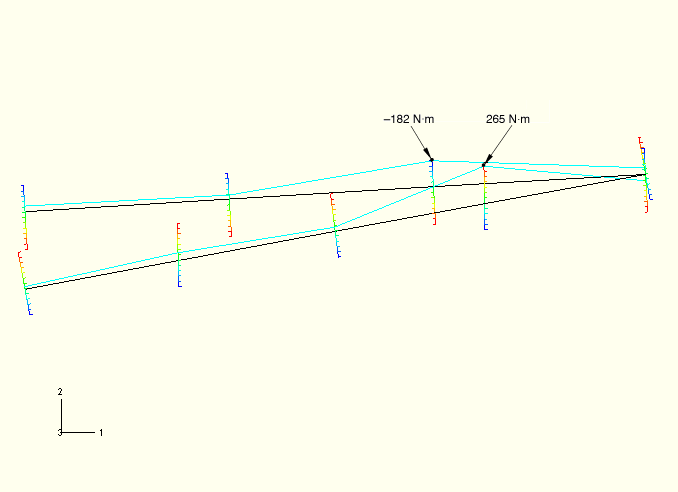
ABAQUS can provide output for structural elements in terms of forces and moments acting on the cross-section at a given point. These section forces and moments are defined in the local beam coordinate system. Contour the section moment about the beam 1-axis in the elements in display group MainA. For clarity, reset the view so that the elements are displayed in the 1–2 plane.
To create a “bending moment”-type contour plot:
From the main menu bar, select Result![]() Field Output.
Field Output.
The Field Output dialog box appears; by default, the Primary Variable tab is selected.
Select SM from the list of available output variables; then select SM1 from the component field.
Click OK.
The Select Plot State dialog box appears.
Toggle on Contour, and click OK.
ABAQUS/CAE displays a contour plot of the bending moment about the beam 1-axis. The contour is plotted on the deformed model shape. The deformation scale factor is chosen automatically since geometric nonlinearity was not considered in the analysis.
Open the Common Plot Options dialog box, and select a Uniform deformation scale factor of 1.0.
Color contour plots of this type typically are not very useful for one-dimensional elements such as beams. A more useful plot is a “bending moment”-type plot, which you can produce using the contour options.
From the main menu bar, select Options![]() Contour; or use the Contour Options
Contour; or use the Contour Options ![]() tool in the toolbox.
tool in the toolbox.
The Contour Plot Options dialog box appears; by default, the Basic tab is selected.
In the Contour Type field, toggle on Show tick marks for line elements.
Click OK.
The plot shown in Figure 6–27 appears.
The magnitude of the variable at each node is now indicated by the position at which the contour curve intersects a “tick mark” drawn perpendicular to the element. This “bending moment”-type plot can be used for any variable (not just bending moments) for any one-dimensional element, including trusses and axisymmetric shells as well as beams.