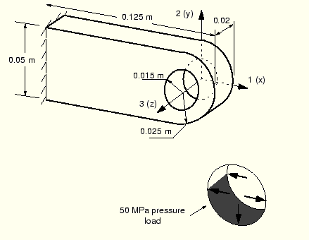
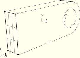
In this example you will use three-dimensional, continuum elements to model the connecting lug shown in Figure 4–14.
The lug is welded firmly to a massive structure at one end. The other end contains a hole. When it is in service, a bolt will be placed through the hole of the lug. You have been asked to determine the static deflection of the lug when a 30 kN load is applied to the bolt in the negative 2-direction. Because the goal of this analysis is to examine the static response of the lug, you should use ABAQUS/Standard as your analysis product. You decide to simplify this problem by making the following assumptions:
Rather than include the complex bolt-lug interaction in the model, you will use a distributed pressure over the bottom half of the hole to load the connecting lug (see Figure 4–14).
You will neglect the variation of pressure magnitude around the circumference of the hole and use a uniform pressure.
The magnitude of the applied uniform pressure will be 50 MPa: 30 kN/ (2 × 0.015 m × 0.02 m).
After examining the static response of the lug, you will modify the model and use ABAQUS/Explicit to study the transient dynamic effects resulting from sudden loading of the lug.
In this section we discuss how to use ABAQUS/CAE to create the entire model for this simulation. A Python script is provided in “Connecting lug,” Section A.2. When this script is run through ABAQUS/CAE, it creates the complete analysis model for this problem. Run this script if you encounter difficulties following the instructions given below or if you wish to check your work. Instructions on how to fetch and run the script are given in Appendix A, “Example Files.”
If you do not have access to ABAQUS/CAE or another preprocessor, the input file required for this problem can be created manually, as discussed in “Example: connecting lug,” Section 4.3 of Getting Started with ABAQUS/Standard: Keywords Version.
Starting ABAQUS/CAE
Start ABAQUS/CAE by typing
abaqus caeat the operating system prompt, where abaqus is the command used to run ABAQUS on your system. Select Create Model Database from the Start Session dialog box that appears.
Defining the model geometry
As always, the first step in creating the model is to define its geometry. In this example you will create a three-dimensional, deformable body with a solid, extruded base feature. You will first sketch the two-dimensional profile of the lug and then extrude it.
You need to decide what system of units to use in your model. The SI system of meters, seconds, and kilograms is recommended; but you can use another system if you prefer.
To create a part:
In the Model Tree, double-click the Parts container to create a new part. From the Create Part dialog box that appears, name the part Lug, and accept the default settings of a three-dimensional, deformable body and a solid, extruded base feature. In the Approximate size text field, type 0.250. This value is twice the largest dimension of the part. Click Continue to exit the Create Part dialog box.
Use the dimensions given in Figure 4–14 to sketch the profile of the lug. The following possible approach can be used:
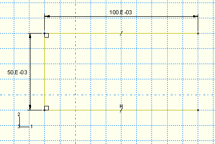
Create an arbitrary rectangle using the Create Lines: Rectangle tool. Delete the right vertical edge, and assign an Equal length constraint to the top and bottom edges using the constraints tool ![]() . Use the dimensions tool
. Use the dimensions tool ![]() to adjust the profile so that it is 0.100 m long × 0.050 m wide, as shown in Figure 4–15.
to adjust the profile so that it is 0.100 m long × 0.050 m wide, as shown in Figure 4–15.
Note:
The figures in this section include dimensions and constraints for the purpose of controlling the shape of the sketch. As seen previously, these tools are accessible from the Sketcher toolbox. These tools are also accessible by selecting Add![]() Constraint and Add
Constraint and Add![]() Dimension, respectively, from the main menu bar.
Dimension, respectively, from the main menu bar.
You can edit the dimension values as you add them to the sketch, or you can edit the value of existing dimensions by selecting Edit![]() Dimension from the main menu bar or by using the Edit Dimension
Dimension from the main menu bar or by using the Edit Dimension ![]() tool.
tool.
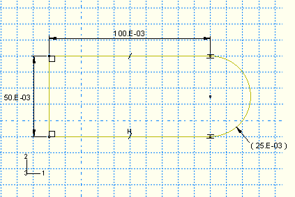
Close the profile by adding a semicircular arc, as shown in Figure 4–16, using the Create Arc: Thru 3 points tool, ![]() .
.
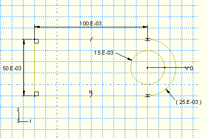
Sketch a circle of radius 0.015 m, as shown in Figure 4–17, using the Create Circle: Center and Perimeter tool, ![]() .
.
The perimeter point of the circle should be on the same horizontal plane as the circle center point (as in Figure 4–17). If these two points do not line up correctly, dimension the vertical distance between the center of the circle and the perimeter point so that the distance is 0.
Note: When you mesh a part, ABAQUS/CAE places nodes wherever vertices appear along an edge; therefore, the location of the vertex on the circumference of the circle influences the final mesh. Placing it on the same horizontal plane as the center point results in a high-quality mesh.
Click Done in the prompt area when you are finished sketching the profile.
The Edit Base Extrusion dialog box appears. To complete the part definition, you must specify the distance over which the profile will be extruded.
In the dialog box, enter an extrusion distance of 0.020 m.
ABAQUS/CAE exits the Sketcher and displays the part.
Defining the material and section properties
The next step in creating the model involves defining and assigning material and section properties to the part. Each region of a deformable body must refer to a section property, which includes the material definition. In this model you will create a single linear elastic material with a Young's modulus E = 200 GPa and Poisson's ratio ![]() = 0.3.
= 0.3.
To define material properties:
In the Model Tree, double-click the Materials container to create a new material definition.
In the material editor that appears, name the material Steel and select Mechanical![]() Elasticity
Elasticity![]() Elastic. Enter 200.0E9 for the Young's Modulus and 0.3 for the Poisson's Ratio. Click OK.
Elastic. Enter 200.0E9 for the Young's Modulus and 0.3 for the Poisson's Ratio. Click OK.
To define section properties:
In the Model Tree, double-click the Sections container to create a new section definition. Accept the default solid, homogeneous section type; and name the section LugSection. Click Continue.
In the Edit Section dialog box that appears, accept Steel as the material and 1 as the Plane stress/strain thickness, and click OK.
To assign section properties:
In the Model Tree, expand the Lug item underneath the Parts container and double-click Section Assignments in the list of part attributes that appears.
Select the entire part as the region to which the section will be assigned by clicking on it. When the part is highlighted, click Done in the prompt area.
In the Edit Section Assignment dialog box that appears, accept LugSection as the section definition, and click OK.
Creating an assembly
An assembly contains all the geometry included in the finite element model. Each ABAQUS/CAE model contains a single assembly. The assembly is initially empty, even though you have already created a part. You will create an instance of the part in the Assembly module to include it in your model.
To instance a part:
In the Model Tree, expand the Assembly container and double-click Instances in the list that appears to create an instance of the part.
In the Create Instance dialog box, select Lug from the Parts list and click OK.
The model is oriented by default so that the global 1-axis lies along the length of the lug, the global 2-axis is vertical, and the global 3-axis lies in the thickness direction.
Defining steps and specifying output requests
You will now define the analysis steps. Since interactions, loads, and boundary conditions can be step dependent, analysis steps must be defined before these can be specified. For this simulation you will define a single static, general step. In addition, you will specify output requests for your analysis. These requests will include output to the output database (.odb) file.
To define a step:
In the Model Tree, double-click the Steps container to create an analysis step. In the Create Step dialog box that appears, name the step LugLoad and accept the General procedure type. From the list of available procedure options, accept Static, General. Click Continue.
In the Edit Step dialog box that appears, enter the following step description: Apply uniform pressure to the hole. Accept the default settings, and click OK.
To specify output requests to the .odb file:
In the Model Tree, click mouse button 3 on the Field Output Requests container and select Manager from the menu that appears.
In the Field Output Requests Manager that appears, select the cell labeled Created in the column labeled LugLoad if it is not already selected. The information at the bottom of the dialog box indicates that preselected default field output requests have been made for this step.
On the right side of the dialog box, click Edit to change the field output requests. In the Edit Field Output Request dialog box that appears:
Click the arrow next to Stresses to show the list of available stress output. Accept the default selection of stress components and invariants.
Under Forces/Reactions, request only the reaction forces (selected by default) by toggling off concentrated force and moment output.
Toggle off Strains and Contact.
Accept the default Displacement/Velocity/Acceleration output.
Click OK, and click Dismiss to close the Field Output Requests Manager.
Delete all history output requests. In the Model Tree, click mouse button 3 on the History Output Requests container and select Manager to open the History Output Requests Manager. In the History Output Requests Manager, select the cell labeled Created in the column labeled LugLoad if it is not already selected. At the bottom of the dialog box, click Delete and click Yes in the warning dialog box that appears. Click Dismiss to close the History Output Requests Manager.
Prescribing boundary conditions and applied loads
In this model the left-hand end of the connecting lug needs to be constrained in all three directions. This region is where the lug is attached to its parent structure (see Figure 4–18). In ABAQUS/CAE boundary conditions are applied to geometric regions of a part rather than to the finite element mesh itself. This association between boundary conditions and part geometry makes it very easy to vary the mesh without having to respecify the boundary conditions. The same holds true for load definitions.
To prescribe boundary conditions:
In the Model Tree, double-click the BCs container to prescribe boundary conditions on the model. In the Create Boundary Condition dialog box that appears, name the boundary condition Fix left end, and select LugLoad as the step in which it will be applied (since it is a fixed condition, it can be applied either in the initial step or the analysis step; here we choose the analysis step for convenience). Accept Mechanical as the category and Symmetry/Antisymmetry/Encastre as the type. Click Continue.
You may need to rotate the view to facilitate your selection in the following steps. Select View![]() Rotate from the main menu bar (or use the
Rotate from the main menu bar (or use the ![]() tool from the toolbar) and drag the cursor over the virtual trackball in the viewport. The view rotates interactively; try dragging the cursor inside and outside the virtual trackball to see the difference in behavior. Click mouse button 2 to exit the rotate view tool before proceeding.
tool from the toolbar) and drag the cursor over the virtual trackball in the viewport. The view rotates interactively; try dragging the cursor inside and outside the virtual trackball to see the difference in behavior. Click mouse button 2 to exit the rotate view tool before proceeding.
Select the left end of the lug (indicated in Figure 4–18) using the cursor. Click Done in the prompt area when the appropriate region is highlighted in the viewport, and toggle on ENCASTRE in the Edit Boundary Condition dialog box that appears. Click OK to apply the boundary condition.
Arrows appear on the face indicating the constrained degrees of freedom. The encastre boundary condition constrains all active structural degrees of freedom in the region specified; after the part is meshed and the job is created, this constraint will be applied to all the nodes that occupy the region.
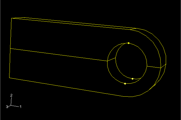
The lug carries a pressure of 50 MPa distributed around the bottom half of the hole. To apply the load correctly, however, the part must first be partitioned (i.e., divided) so that the hole is composed of two regions: a top half and a bottom half.
You use the Partition toolset to divide a part or assembly into regions. Partitioning is used for many reasons; it is commonly used for the purposes of defining material boundaries, indicating the location of loads and constraints (as in this example), and refining the mesh. An example of the use of partitioning for meshing purposes is discussed in the next section. For more information on partitioning, see Chapter 44, “The Partition toolset,” of the ABAQUS/CAE User's Manual.
Dependent part instances cannot be modified at the assembly level (e.g., they cannot be partitioned in an assembly-level module). The reason for this restriction is that all dependent instances of a part must have identical geometry so they can share the same mesh topology as the original part. Thus, any change to a dependent part instance has to be made to the original part itself (i.e., at the part level). In contrast, independent part instances may be partitioned at the assembly level. In this example a dependent part instance (the default) was created; the corresponding partitioning instructions follow.
To partition a dependent part instance:
In the Model Tree, double-click the Lug item in the Parts container to make it current.
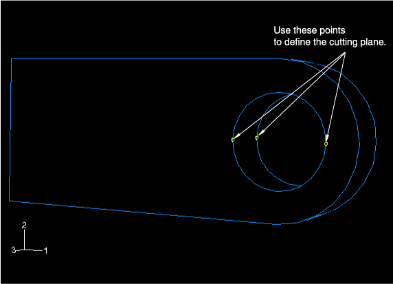
Use the Partition Cell: Define Cutting Plane tool ![]() to divide the part in half. Use the 3 Points method to define the cutting plane. When you are prompted to select a point, ABAQUS/CAE highlights the points you can select: vertices, datum points, edge midpoints, or arc centers. In this model the points used to define the cutting plane are indicated in Figure 4–19. Again, you may need to rotate the view to facilitate your selection.
to divide the part in half. Use the 3 Points method to define the cutting plane. When you are prompted to select a point, ABAQUS/CAE highlights the points you can select: vertices, datum points, edge midpoints, or arc centers. In this model the points used to define the cutting plane are indicated in Figure 4–19. Again, you may need to rotate the view to facilitate your selection.
Click Create Partition in the prompt area after you have finished selecting the points.
To apply a pressure load:
In the Model Tree, double-click the Loads container to prescribe the pressure load. In the Create Load dialog box that appears, name the load Pressure load and select LugLoad as the step in which it will be applied. Select Mechanical as the category and Pressure as the type. Click Continue.
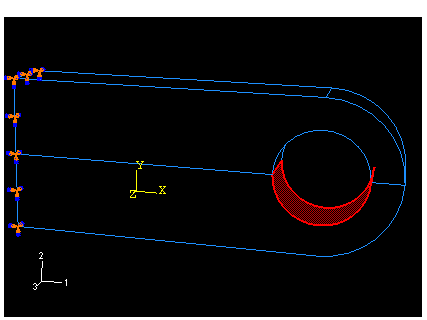
Select the surface associated with the bottom half of the hole using the cursor; the region is highlighted in Figure 4–20. When the appropriate surface is selected, click Done in the prompt area.
Specify a uniform pressure of 5.0E7 in the Edit Load dialog box, accept the default Amplitude, and click OK to apply the load.
Arrows appear on the nodes of the face indicating the applied load.
Designing the mesh: partitioning and creating the mesh
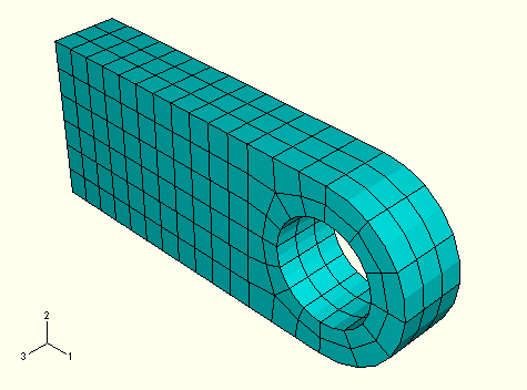
You need to consider the type of element that will be used before you start building the mesh for a particular problem. For example, a suitable mesh design that uses quadratic elements may very well be unsuitable if you change to linear, reduced-integration elements. For this example use 20-node hexahedral elements with reduced integration (C3D20R). Once you have selected the element type, you can design the mesh for the connecting lug. The most important decision regarding the mesh design for this example is how many elements to use around the circumference of the lug's hole. A possible mesh for the connecting lug is shown in Figure 4–21.
Another thing to consider when designing a mesh is the type of results you want from the simulation. The mesh in Figure 4–21 is rather coarse and, therefore, unlikely to yield accurate stresses. Four quadratic elements per 90° is the minimum number that should be considered for a problem such as this one; using twice that many is recommended to obtain reasonably accurate stress results. However, this mesh should be adequate to predict the overall level of deformation in the lug under the applied loads, which is what you were asked to determine. The influence of increasing the mesh density used in this simulation is discussed in “Mesh convergence,” Section 4.4.
ABAQUS/CAE offers a variety of meshing techniques to mesh models of different topologies. The different meshing techniques provide varying levels of automation and user control. The following three types of mesh generation techniques are available:
Structured meshing
Structured meshing applies preestablished mesh patterns to particular model topologies. Complex models must generally be partitioned into simpler regions to use this technique.
Swept meshing
Swept meshing extrudes an internally generated mesh along a sweep path or revolves it around an axis of revolution. Like structured meshing, swept meshing is limited to models with specific topologies and geometries.
Free meshing
The free meshing technique is the most flexible meshing technique. It uses no preestablished mesh patterns and can be applied to almost any model shape.
When you enter the Mesh module, ABAQUS/CAE color codes regions of the model according to the methods it will use to generate a mesh:
Green indicates that a region can be meshed using structured methods.
Yellow indicates that a region can be meshed using sweep methods.
Pink indicates that a region can be meshed using the free method.
Orange indicates that a region cannot be meshed using the default element shape assignment and must be partitioned further.
Dependent part instances are colored blue at the assembly level. You must switch to a part-level view to mesh a dependent part instance.
In this problem you will create a structured mesh. You will find that the model must first be partitioned further to use this mesh technique. After the partitions have been created, a global part seed will be assigned and the mesh will be created.
To partition the lug:
In the Model Tree, expand the Lug item underneath the Parts container and double-click Mesh in the menu that appears.
The part is colored yellow initially, indicating that with the default set of mesh controls, a hexahedral mesh can be created only using a swept mesh technique. Additional cell partitions are required to permit structured meshing. Two partitions will be created. The first partition permits structured meshing to be used, and the second improves the overall quality of the mesh.
Note: The Object field that appears in the context bar automatically displays the part so that you can partition the geometry directly within the Mesh module. The ability to switch between individual parts and the model assembly within the same module is available only in the Mesh module. This feature allows you to partition both dependent and independent part instances in the same module for the purpose of meshing. In all other modules, partitioning must be done strictly at the part level for dependent instances (as was done earlier when the pressure load was applied) or at the assembly level for independent part instances.
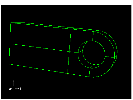
Partition both regions of the lug vertically by defining a cutting plane through the three points shown in Figure 4–22 (use [Shift]+Click to select both regions simultaneously).
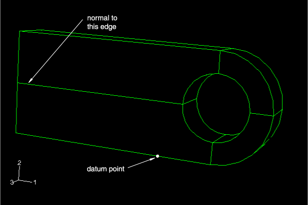
Select Tools![]() Datum from the main menu bar, and create a datum point 0.075 m from the left end of the lug (as shown in Figure 4–23) using the Offset from point method.
Datum from the main menu bar, and create a datum point 0.075 m from the left end of the lug (as shown in Figure 4–23) using the Offset from point method.
Create the second vertical partition by defining a cutting plane through the datum point you just created and normal to the centerline of the lug (as shown in Figure 4–23).
To assign a global part seed and create the mesh:
From the main menu bar, select Seed![]() Part, and specify a target global element size of 0.007. Seeds appear on all the edges.
Part, and specify a target global element size of 0.007. Seeds appear on all the edges.
From the main menu bar, select Mesh![]() Element Type to choose the element type for the part. Because of the partitions you have created, the part is now composed of several regions.
Element Type to choose the element type for the part. Because of the partitions you have created, the part is now composed of several regions.
Use the cursor to draw a box around the entire part and, thus, select all regions of the part. Click Done in the prompt area.
In the Element Type dialog box that appears, select the Standard element library, 3D Stress family, Quadratic geometric order, and Hex, Reduced integration element. Click OK to accept the choice of C3D20R as the element type.
Note: If you are using the ABAQUS Student Edition, using second-order elements with a global seed size of 0.007 results in a mesh that exceeds the model size limits of the product. Either use first-order elements (C3D8R) with a global seed size of 0.007 or second-order elements with a global seed size of 0.01.
From the main menu bar, select Mesh![]() Part. Click Yes in the prompt area to mesh the part instance.
Part. Click Yes in the prompt area to mesh the part instance.
Creating, running, and monitoring a job
At this point the only task remaining to complete the model is defining the job. The job can then be submitted from within ABAQUS/CAE and the solution progress monitored interactively.
Before continuing, rename the model to Elastic by clicking mouse button 3 on Model-1 in the Model Tree and selecting Rename from the menu that appears. This model will later form the basis of the model used in the lug example discussed in Chapter 10, “Materials.”
To create a job:
In the Model Tree, double-click the Jobs container to create a job. Name the job Lug, and click Continue.
In the Edit Job dialog box, enter the following description: Linear Elastic Steel Connecting Lug.
Accept the default job settings, and click OK.
Save your model in a model database file named Lug.cae.
To run the job:
In the Model Tree, click mouse button 3 on the job named Lug and select Submit to submit your job for analysis.
A dialog box appears to warn you that history output has not been requested for the LugLoad step. Click Yes to continue with the job submission.
In the Model Tree, click mouse button 3 on the job named Lug and select Monitor from the menu that appears to open the job monitor.
At the top of the dialog box, a summary of the solution progress is included. This summary is updated continuously as the analysis progresses. Any errors and/or warnings that are encountered during the analysis are noted in the appropriate tabbed pages. If any errors are encountered, correct the model and rerun the simulation. Be sure to investigate the cause of any warning messages and take appropriate action; recall that some warning messages can be ignored safely while others require corrective action.
When the job has completed, click Dismiss to close the job monitor.
In the Model Tree, click mouse button 3 on the job named Lug and select Results to enter the Visualization module and automatically open the output database (.odb) file created by this job. Alternatively, from the Module list located under the toolbar, select Visualization to enter the Visualization module; open the .odb file by selecting File![]() Open from the main menu bar and double-clicking on the appropriate file.
Open from the main menu bar and double-clicking on the appropriate file.
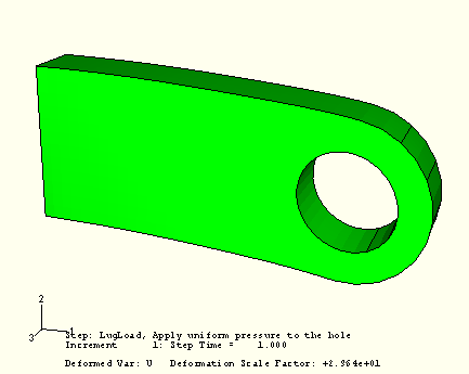
Plotting the deformed shape
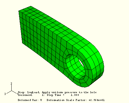
From the main menu bar, select Plot![]() Deformed Shape; or use the
Deformed Shape; or use the ![]() tool in the toolbox. Figure 4–25 displays the deformed model shape at the end of the analysis. What is the displacement magnification level?
tool in the toolbox. Figure 4–25 displays the deformed model shape at the end of the analysis. What is the displacement magnification level?
Changing the view
The default view is isometric. You can change the view using the options in the View menu or the view tools in the toolbar. You can also specify a view by entering values for rotation angles, viewpoint, zoom factor, or fraction of viewport to pan.
To specify the view:
From the main menu bar, select View![]() Specify.
Specify.
The Specify View dialog box appears.
From the list of available methods, select Viewpoint.
In the Viewpoint method, you enter three values representing the X-, Y-, and Z-position of an observer. You can also specify an up vector. ABAQUS positions your model so that this vector points upward.
Enter the X-, Y-, and Z-coordinates of the viewpoint vector as 1, 1, 3 and the coordinates of the up vector as 0, 1, 0.
Click OK.
ABAQUS/CAE displays your model in the specified view, as shown in Figure 4–26.
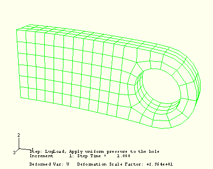
Visible edges
Several options are available for choosing which edges will be visible in the model display. The previous plots show all exterior edges of the model; Figure 4–27 displays only feature edges.
To display only feature edges:
From the main menu bar, select Options![]() Common.
Common.
The Common Plot Options dialog box appears.
Click the Basic tab if it is not already selected.
From the Visible Edges options, choose Feature edges.
Click Apply.
The deformed plot in the current viewport changes to display only feature edges, as shown in Figure 4–27.
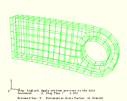
Render style
A shaded plot is a filled plot in which a lightsource appears to be directed at the model. This is the default render style and can be very useful when viewing complex three-dimensional models. Three other render styles provide additional display options: wireframe, hidden line, and filled. You can select a render style from the Common Plot Options dialog box or from the render style tools on the toolbar: wireframe ![]() , hidden line
, hidden line ![]() , filled
, filled ![]() , and shaded
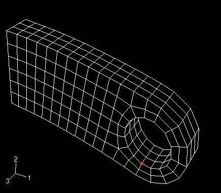
, and shaded ![]() . To display the wireframe plot shown in Figure 4–28, select Exterior edges in the Common Plot Options dialog box, click OK to close the dialog box, and select wireframe plotting by clicking the
. To display the wireframe plot shown in Figure 4–28, select Exterior edges in the Common Plot Options dialog box, click OK to close the dialog box, and select wireframe plotting by clicking the ![]() tool. All subsequent plots will be displayed in the wireframe render style until you select another render style.
tool. All subsequent plots will be displayed in the wireframe render style until you select another render style.
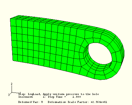
A wireframe model showing internal edges can be visually confusing for complex three-dimensional models. You can use the other render style tools to select the hidden line and filled render styles, shown in Figure 4–29 and Figure 4–30, respectively. These render styles are more useful when viewing complex three-dimensional models.
Contour plots
Contour plots display the variation of a variable across the surface of a model. You can create filled or shaded contour plots of field output results from the output database.
To generate a contour plot of the Mises stress:
From the main menu bar, select Plot![]() Contours
Contours![]() On Deformed Shape.
On Deformed Shape.
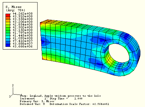
The filled contour plot shown in Figure 4–31 appears.
The Mises stress, S Mises, indicated in the legend title is the default variable chosen by ABAQUS for this analysis. You can select a different variable to plot.
From the main menu bar, select Result![]() Field Output.
Field Output.
The Field Output dialog box appears; by default, the Primary Variable tab is selected.
From the list of available output variables, select a new variable to plot.
Click OK.
The contour plot in the current viewport changes to reflect your selection.
ABAQUS/CAE offers many options to customize contour plots. To see the available options, click the Contour Options ![]() tool in the toolbox. By default, ABAQUS/CAE automatically computes the minimum and maximum values shown in your contour plots and evenly divides the range between these values into 12 intervals. You can control the minimum and maximum values ABAQUS/CAE displays (for example, to examine variations within a fixed set of bounds), as well as the number of intervals.
tool in the toolbox. By default, ABAQUS/CAE automatically computes the minimum and maximum values shown in your contour plots and evenly divides the range between these values into 12 intervals. You can control the minimum and maximum values ABAQUS/CAE displays (for example, to examine variations within a fixed set of bounds), as well as the number of intervals.
To generate a customized contour plot:
In the Basic tabbed page of the Contour Plot Options dialog box, drag the Contour Intervals slider to change the number of intervals to nine.
In the Limits tabbed page of the Contour Plot Options dialog box, choose Specify beside Max; then enter a maximum value of 400E+6.
Choose Specify beside Min; then enter a minimum value of 60E+6.
Click OK.
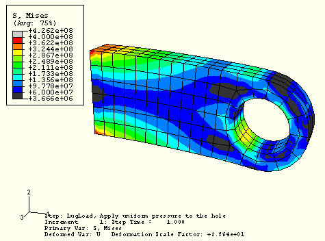
ABAQUS/CAE displays your model with the specified contour option settings, as shown in Figure 4–32 (this figure shows Mises stress; your plot will show whichever output variable you have chosen). These settings remain in effect for all subsequent contour plots until you change them or reset them to their default values.
Displaying contour results on interior surfaces
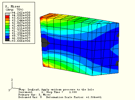
You can cut your model such that interior surfaces are made visible. For example, you may want to examine the stress distribution in the interior of a part. View cuts can be created for such purposes. Here, a simple planar cut is made through the lug to view the Mises stress distribution through the thickness of the part.
To create a view cut:
From the main menu bar, select Tools![]() View Cut
View Cut![]() Create.
Create.
In the dialog box that appears, accept the default name and shape. Enter 0,0,0 as the Origin of the plane (i.e., a point through which the plane will pass), 1,0,1 as the Normal axis to the plane, and 0,1,0 as Axis 2 of the plane.
Click OK to close the dialog box and to make the view cut.
The view appears as shown in Figure 4–33.
From the main menu bar, select ToolsTo view the full model again, toggle off Cut-4 in the View Cut Manager.
For more information on view cuts, see Chapter 34, “Cutting through a model,” of the ABAQUS/CAE User's Manual.
Maximum and minimum values
The maximum and minimum values of a variable in a model can be determined easily.
To display the minimum and maximum values of a contour variable:
From the main menu bar, select Viewport![]() Viewport Annotation Options; then click the Legend tab in the dialog box that appears.
Viewport Annotation Options; then click the Legend tab in the dialog box that appears.
The Legend options become available.
Toggle on Show min/max values.
Click OK.
The contour legend changes to report the minimum and maximum contour values.
One of the goals of this workshop was to determine the deflection of the lug in the negative 2-direction. You will contour the displacement component of the lug in the 2-direction to determine its peak displacement in the vertical direction. In the Contour Plot Options dialog box, click Defaults to reset the minimum and maximum contour values and the number of intervals to their default values before proceeding.
To contour the displacement of the connecting lug in the 2-direction:
From the main menu bar, select Result![]() Field Output.
Field Output.
The Field Output dialog box appears; by default, the Primary Variable tab is selected.
From the list of available output variables, select U.
From the list of available components, select U2.
Click OK.
Displaying a subset of the model
By default, ABAQUS/CAE displays your entire model; however, you can choose to display a subset of your model called a display group. This subset can contain any combination of part instances, geometry (cells, faces, or edges), elements, nodes, and surfaces from the current model or output database. For the connecting lug model you will create a display group consisting of the elements at the bottom of the hole. Since a pressure load was applied to this region, an internal set is created by ABAQUS that can be used for visualization purposes.
To display a subset of the model:
In the Results Tree, double-click Display Groups.
The Create Display Group dialog box opens.
From the Item list, select Elements. From the Selection Method list, select Internal sets.
Once you have selected these items, the list on the right-hand side of the Create Display Group dialog box shows the available selections.
Using this list, identify the set that contains the elements at the bottom of the hole. Toggle on Highlight items in viewport below the list so that the outlines of the elements in the selected set are highlighted in red.
When the highlighted set corresponds to the group of elements at the bottom of the hole, click Replace ![]() to replace the current model display with this element set.
to replace the current model display with this element set.
ABAQUS/CAE displays the specified subset of your model.
Click Dismiss to close the Create Display Group dialog box.
When creating an ABAQUS model, you may want to determine the face labels for a solid element. For example, you may want to verify that the correct load ID was used when applying pressure loads or when defining surfaces for contact. In such situations you can use the Visualization module to display the mesh after you have run a datacheck analysis that creates an output database file.
To display the face identification labels and element numbers on the undeformed model shape:
From the main menu bar, select Options![]() Common.
Common.
The Common Plot Options dialog box appears.
Set the render style to filled; all visible element edges will be displayed for convenience.
Toggle on Filled under Render Style.
Toggle on All edges under Visible Edges.
Click the Labels tab, and toggle on Show element labels and Show face labels.
Click Apply to apply the plot options.
From the main menu bar, select Plot![]() Undeformed Shape; or use the
Undeformed Shape; or use the ![]() tool in the toolbox.
tool in the toolbox.
ABAQUS/CAE displays the element and face identification labels in the current display group.
Click Defaults in the Common Plot Options dialog box to restore the default plot settings and then click OK to close the dialog box.
Generating tabular data reports for subsets of the model
In the overhead hoist frame problem tabular output data were generated for the entire model. For more complicated models it is convenient to write these data for selected regions of the model. This is achieved using display groups in conjunction with the report generation feature. For the connecting lug problem we will generate the following tabular data reports:
Stresses in the elements at the built-in end of the lug (to determine the maximum stress in the lug)
Reaction forces at the built-in end of the lug (to check that the reaction forces at the constraints balance the applied loads)
Vertical displacements at the bottom of the hole (to determine the deflection of the lug when the load is applied)
Since we did not create geometry sets corresponding to these regions, each of these reports will be generated using display groups whose contents are selected in the viewport. Thus, begin by creating and saving display groups for each region of interest.
To create and save a display group containing the elements at the built-in end:
In the Results Tree, double-click Display Groups.
In the Create Display Group dialog box, select All from the Item list, and click Replace ![]() to replace the contents of the viewport with the entire model.
to replace the contents of the viewport with the entire model.
Choose Elements from the Item list and Pick from viewport as the selection method.
In the prompt area, set the selection method to by angle; and click the built-in face of the lug. Click Done when all the elements at the built-in face of the lug are highlighted in the viewport. In the Create Display Group dialog box, click Replace ![]() followed by Save As. Save the display group as built-in elements.
followed by Save As. Save the display group as built-in elements.
To create and save a display group containing the nodes at the built-in end:
In the Create Display Group dialog box, choose Nodes from the Item list and Pick from viewport as the selection method.
In the prompt area, set the selection method to by angle; and click the built-in face of the lug. Click Done when all the nodes on the built-in face of the lug are highlighted in the viewport. In the Create Display Group dialog box, click Replace ![]() followed by Save As. Save the display group as built-in nodes.
followed by Save As. Save the display group as built-in nodes.
To create and save a display group containing the nodes at the bottom of the hole:
In the Create Display Group dialog box, select All from the item list, and click Replace ![]() to reset the active display group to include the entire model.
to reset the active display group to include the entire model.
In the Create Display Group dialog box, choose Nodes from the Item list and Pick from viewport as the selection method.
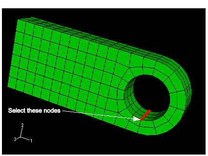
In the prompt area, set the selection method to individually; and select the nodes at the bottom of the hole in the lug, as indicated in Figure 4–34. Click Done when all the nodes on the bottom of the hole are highlighted in the viewport. In the Create Display Group dialog box, click Replace ![]() followed by Save As. Save the display group as nodes at hole bottom.
followed by Save As. Save the display group as nodes at hole bottom.
Now generate the reports.
To generate field data reports:
In the Results Tree, click mouse button 3 on built-in elements underneath the Display Groups container. In the menu that appears, select Plot to make it the current display group.
From the main menu bar, select Report![]() Field Output.
Field Output.
In the Variable tabbed page of the Report Field Output dialog box, accept the default position labeled Integration Point. Click the triangle next to S: Stress components to expand the list of available variables. From this list, select Mises and the six individual stress components: S11, S22, S33, S12, S13, and S23.
In the Setup tabbed page, name the report Lug.rpt. In the Data region at the bottom of the page, toggle off Column totals.
Click Apply.
In the Results Tree, click mouse button 3 on built-in nodes underneath the Display Groups container. In the menu that appears, select Plot to make it the current display group. (To see the nodes, toggle on Show node symbols in the Common Plot Options dialog box.)
In the Variable tabbed page of the Report Field Output dialog box, change the position to Unique Nodal. Toggle off S: Stress components, and select RF1, RF2, and RF3 from the list of available RF: Reaction force variables.
In the Data region at the bottom of the Setup tabbed page, toggle on Column totals.
Click Apply.
In the Results Tree, click mouse button 3 on nodes at hole bottom underneath the Display Groups container. In the menu that appears, select Plot to make it the current display group.
In the Variable tabbed page of the Report Field Output dialog box, toggle off RF: Reaction force, and select U2 from the list of available U: Spatial displacement variables.
In the Data region at the bottom of the Setup tabbed page, toggle off Column totals.
Click OK.
Open the file Lug.rpt in a text editor. A portion of the table of element stresses is shown below. The element data are given at the element integration points. The integration point associated with a given element is noted under the column labeled Int Pt. The bottom of the table contains information on the maximum and minimum stress values in this group of elements. The results indicate that the maximum Mises stress at the built-in end is approximately 330 MPa. Your results may differ slightly if your mesh is not identical to the one used here.
Field Output Report

Source 1
---------

   ODB: Lug.odb
   Step: LugLoad
   Frame: Increment      1: Step Time =    1.000

Loc 1 : Integration point values from source 1

Output sorted by column "Element Label".

Field Output reported at integration points for part: LUG-1

Element   Int      S.Mises        S.S11        S.S22        S.S33        S.S12
Label     Pt        @Loc 1       @Loc 1       @Loc 1       @Loc 1       @Loc 1
------------------------------------------------------------------------------
        S.S13        S.S23
       @Loc 1       @Loc 1
--------------------------
   31     1    84.0567E+06  76.2075E+06   14.021E+06 -274.446E+03 -26.4339E+06
 -159.756E+03  1.70193E+06
   31     2    88.1108E+06  79.9769E+06  16.7815E+06  5.07167E+06 -30.8241E+06
    3.045E+06  2.20251E+06
   31     3    71.0378E+06  87.4511E+06  30.5433E+06  22.7759E+06 -11.8374E+06
   17.114E+06  1.47033E+06
   31     4    64.3978E+06  76.4473E+06  26.1412E+06  19.0617E+06 -18.6815E+06
  7.36221E+06  411.436E+03
   31     5    48.4688E+06  20.2162E+06  4.20669E+06  68.3536E+03 -25.8284E+06
 -78.8286E+03  1.65403E+06
   31     6    55.6407E+06  21.1693E+06  4.87661E+06  1.46182E+06 -30.2661E+06
  796.514E+03   2.0911E+06
   31     7    25.1732E+06  22.9107E+06  7.96147E+06  5.89815E+06 -10.1069E+06
  4.55755E+06  1.45446E+06
   31     8    32.8268E+06   19.928E+06  6.76018E+06  4.88587E+06 -16.9708E+06
   1.9631E+06  378.549E+03
    .
    .
  198     1    239.655E+06 -247.046E+06 -20.9897E+06 -13.4824E+06  -38.331E+06
  7.48079E+06  -1.1505E+06
  198     2    237.839E+06 -235.534E+06 -13.8995E+06  2.83029E+06  -33.891E+06
 -1.25472E+06 -1.57941E+06
  198     3    190.507E+06 -228.049E+06 -53.1236E+06 -51.1938E+06 -37.0096E+06
  20.3556E+06 -419.555E+03
  198     4    219.144E+06 -259.016E+06 -65.4028E+06  -61.292E+06 -30.1529E+06
   48.227E+06 -2.60239E+06
  198     5    322.607E+06 -330.074E+06 -2.82071E+06 -14.7802E+06 -12.9162E+06
   9.1461E+06 -189.416E+03
  198     6    320.169E+06 -316.345E+06  1.80108E+06  4.87007E+06 -9.15387E+06
 -4.10769E+06 -1.03378E+06
  198     7    300.073E+06 -364.931E+06 -95.1687E+06 -93.2852E+06 -69.7659E+06
  26.8241E+06 -343.386E+03
  198     8    331.098E+06 -399.004E+06 -109.695E+06 -104.075E+06 -62.7377E+06
  64.3938E+06 -2.63754E+06


  Minimum      25.1732E+06 -399.004E+06 -109.695E+06 -122.144E+06 -72.2982E+06
 -64.4051E+06 -2.63899E+06
      At Element        33          196          198          197           98
           99           99
          Int Pt         8            7            8            8            4
            4            4
  Maximum      331.159E+06  399.073E+06  109.719E+06  122.172E+06 -9.15387E+06
  64.4051E+06    2.639E+06
      At Element        97           99           99           98          196
           97           97
          Int Pt         3            4            4            4            5
            3            3
How does the maximum value of Mises stress compare to the value reported in the contour plot generated earlier? Do the two maximum values correspond to the same point in the model? The Mises stresses shown in the contour plot have been extrapolated to the nodes, whereas the stresses written to the report file for this problem correspond to the element integration points. Therefore, the location of the maximum Mises stress in the report file is not exactly the same as the location of the maximum Mises stress in the contour plot. This difference can be resolved by requesting that stress output at the nodes (extrapolated from the element integration points and averaged over all elements containing a given node) be written to the report file. If the difference is large enough to be of concern, this is an indication that the mesh may be too coarse.
The table listing the reaction forces at the constrained nodes is shown below. The Total entry at the bottom of the table contains the net reaction force components for this group of nodes. The results confirm that the total reaction force in the 2-direction at the constrained nodes is equal and opposite to the applied load of –30 kN in that direction.
Field Output Report

Source 1
---------

   ODB: Lug.odb
   Step: LugLoad
   Frame: Increment      1: Step Time =    1.000

Loc 1 : Nodal values from source 1

Output sorted by column "Node Label".

Field Output reported at nodes for part: LUG-1

            Node          RF.RF1          RF.RF2          RF.RF3
           Label          @Loc 1          @Loc 1          @Loc 1
----------------------------------------------------------------
               3    -60.6106E-03        -118.486    -31.3131E-03
               4    -60.6102E-03        -118.486     31.3133E-03
               6         538.194         289.574         382.416
               7         538.194         289.574        -382.416
              11        -538.255         289.563        -382.329
       .
       .
            1334     5.90186E+03         216.099     1.63004E+03
            1336     6.60254E+03     1.81494E+03     -45.543E-06
            1337     9.81613E+03         692.328        -791.954
            1339     6.35335E+03      1.7276E+03        -331.533
            1340     5.90186E+03         216.098    -1.63004E+03


  Minimum           -9.81734E+03        -264.368    -1.63023E+03
         At Node             953             258             950

  Maximum            9.81613E+03     1.81556E+03     1.63022E+03
         At Node            1337             951             956

           Total    -1.12979E-03     30.0000E+03     61.9937E-06
The table showing the displacements of the nodes along the bottom of the hole (listed below) indicates that the bottom of the hole in the lug has displaced about 0.3 mm. Field Output Report
Source 1
---------
ODB: Lug.odb
Step: LugLoad
Frame: Increment 1: Step Time = 1.000
Loc 1 : Nodal values from source 1
Output sorted by column "Node Label".
Field Output reported at nodes for part: LUG-1
Node U.U2
Label @Loc 1
--------------------------------
23 -314.158E-06
24 -314.158E-06
143 -314.2E-06
144 -314.2E-06
1522 -314.163E-06
1526 -314.211E-06
1529 -314.163E-06
Minimum -314.211E-06
At Node 1526
Maximum -314.158E-06
At Node 23
You will now evaluate the dynamic response of the lug when the same load is applied suddenly. Of special interest is the transient response of the lug. You will have to modify the model for the ABAQUS/Explicit analysis. Before proceeding, copy the existing model to a new model named Explicit. Make all subsequent changes to the Explicit model (you may want to collapse the Elastic model to avoid confusion). Before running the job you will need to add a density definition to the material model, change the step type, and change the element type. In addition, you should make modifications to the field output requests.
To modify the model:
Edit the material definition for Steel to include a mass density of 7800.
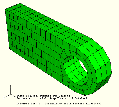
Replace the static step named LugLoad with a dynamic, explicit step. Change the step description to Dynamic lug loading, and enter 0.005 s for the time period of the step.
Edit the field output request named F-Output-1. In the Edit Field Output Request dialog box, enter 40 as the number of equally spaced intervals for saving output.
Change the element type used to mesh the lug. In the Element Type dialog box, select the Explicit element library, 3D Stress family, Linear geometric order, and Hex element. Select enhanced hourglass control for the element. The selected element type is C3D8R.
Create and submit a job named expLug using the model named Explicit.
Monitor the progress of the job.
At the top of the expLug Monitor dialog box, a summary of the solution progress is included. This summary is updated continuously as the analysis progresses. Any errors and/or warnings that are encountered during the analysis are noted in the appropriate tabbed pages. If any errors are encountered, correct the model and rerun the simulation. Be sure to investigate the cause of any warning messages and take appropriate action; recall that some warning messages can be ignored safely while others require corrective action.
In the static analysis performed with ABAQUS/Standard you examined the deformed shape of the lug as well as stress and displacement output. For the ABAQUS/Explicit analysis you can similarly examine the deformed shape, stresses, and displacements in the lug. Because transient dynamic effects may result from a sudden loading, you should also examine the time histories for internal and kinetic energy, displacement, and Mises stress.
Open the output database (.odb) file created by this job.
Plotting the deformed shape
From the main menu bar, select Plot![]() Deformed Shape; or use the
Deformed Shape; or use the ![]() tool in the toolbox. Figure 4–35 displays the deformed model shape at the end of the analysis.
tool in the toolbox. Figure 4–35 displays the deformed model shape at the end of the analysis.
To more clearly see the vibrations in the lug, change the deformation scale factor to 50. In addition, animate the time history of the deformed shape of the lug and decrease the frame rate of the time history animation.
The time history animation of the deformed shape of the lug shows that the suddenly applied load induces vibrations in the lug. Additional insights about the behavior of the lug under this type of loading can be gained by plotting the kinetic energy, internal energy, displacement, and stress in the lug as a function of time. Some of the questions to consider are:
Is energy conserved?
Was large-displacement theory necessary for this analysis?
Are the peak stresses reasonable? Will the material yield?
X–Y plotting
X–Y plots can display the variation of a variable as a function of time. You can create X–Y plots from field and history output.
To create X–Y plots of the internal and kinetic energy as a function of time:
In the Results Tree, expand the History Output container underneath the output database named expLug.odb.
The list of all the variables in the history portion of the output database appears; these are the only history output variables you can plot.
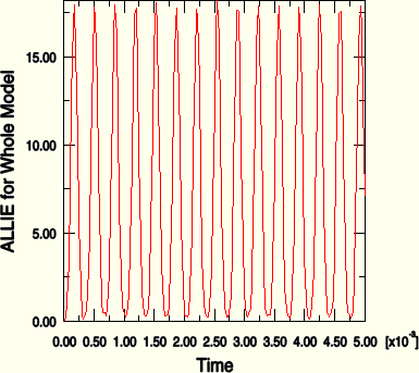
From the list of available output variables, double-click ALLIE to plot the internal energy for the whole model.
ABAQUS reads the data for the curve from the output database file and plots the graph shown in Figure 4–36.
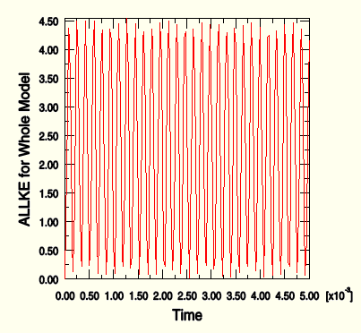
Repeat this procedure to plot ALLKE, the kinetic energy for the whole model (shown in Figure 4–37).
Both the internal energy and the kinetic energy show oscillations that reflect the vibrations of the lug. Kinetic energy is transformed into internal (or strain) energy and vice-versa throughout the simulation. Total energy is conserved (as is expected since the material is linear elastic). This can be seen by plotting ETOTAL together with ALLIE and ALLKE. The value of ETOTAL is approximately zero throughout the course of the analysis. Energy balances in dynamic analysis are discussed further in Chapter 9, “Nonlinear Explicit Dynamics.”
To generate a plot of displacement versus time:
Plot the deformed shape of the lug. In the Results Tree, double-click XY Data.
In the Create XY Data dialog box that appears, toggle on ODB field output and click Continue.
In the XY Data from ODB Field Output dialog box that appears, select Unique Nodal as the type of position from which the X–Y data should be read.
Click the arrow next to U: Spatial displacement and toggle on U2 as the displacement variable for the X–Y data.
Select the Elements/Nodes tab. Choose Pick from viewport as the selection method for identifying the node for which you want X–Y data.
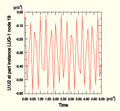
Click Edit Selection. In the viewport, select one of the nodes on the bottom of the hole as shown in Figure 4–38 (if necessary, change the render style to facilitate your selection). Click Done in the prompt area.
Click Plot in the XY Data from ODB Field Output dialog box to plot the nodal displacement as a function of time.
The history of the oscillation, as shown in Figure 4–39, indicates that the displacements are small (relative to the structure's dimensions).
Thus, this problem could have been solved adequately using small-deformation theory. This would have reduced the computational cost of the simulation without significantly affecting the results. Nonlinear geometric effects are discussed further in Chapter 8, “Nonlinearity.”To generate a plot of Mises stress versus time:
Plot the deformed shape of the lug again.
Select the Variables tab in the XY Data from ODB Field Output dialog box. Deselect U2 as the variable for the X–Y data plot.
Change the Position field to Integration Point.
Click the arrow next to S: Stress components and toggle on Mises as the stress variable for the X–Y data.
Select the Elements/Nodes tab. Choose Pick from viewport as the selection method for identifying the node for which you want X–Y data.
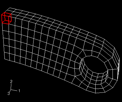
Click Edit Selection. In the viewport, select one of the elements near the built-in end of the lug as shown in Figure 4–40. Click Done in the prompt area.
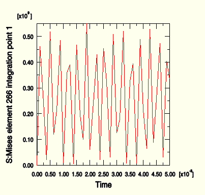
Click Plot in the XY Data from ODB Field Output dialog box to plot the Mises stress at the selected node as a function of time.
The peak Mises stress is on the order of 500 MPa, as shown in Figure 4–41. This value is larger than the typical yield strength of steel. Thus, the material would have yielded before experiencing such a large stress. Material nonlinearity is discussed further in Chapter 10, “Materials.”