This example is divided into three sections. The first section involves calibration of experimental data to determine the material coefficients for the Mullins effect. The second section describes the static response of a solid disc subjected to cyclic deformation induced by contact with a flat rigid surface that represents the road. This kind of test is commonly carried out in the tire industry to investigate the effect of stress softening on the load-deflection behavior of tires. The third section is a continuation of the problem described in the second section and studies the rolling solution of the deformed disc. The rolling is modeled using both a Lagrangian approach that involves rotation of the disc mesh and the steady-state transport capability in ABAQUS/Standard (*STEADY STATE TRANSPORT) that obtains the steady-state solution of the rolling disc using more of an Eulerian approach. This example also illustrates the enhanced hourglass control capability in ABAQUS.

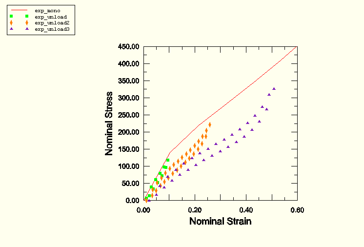
The first step in using the Mullins effect material model is calibration of test data. Figure 3.1.7–1 shows a typical set of uniaxial tension test data for filled rubber. These data are representative of a class of rubber materials that is used in the tire industry and have been provided by Cooper Tire and Rubber Company. The bold curve labeled exp_mono represents the primary behavior of the rubber material that would be obtained from a monotonic test to a certain deformation level. These data are provided to ABAQUS using the *UNIAXIAL TEST DATA option along with the *HYPERELASTIC, TEST DATA INPUT option. In this example the Yeoh material model is used for calibrating the primary material behavior. Reduced polynomial models, such as the Yeoh model, provide a better fit when limited test data are available, as is the case here. The unloading-reloading data, needed to calibrate the Mullins effect coefficients, are provided as stabilized loading/unloading cyclic data from three different maximum strain levels. Although the model for Mullins effect in ABAQUS predicts unloading and reloading from a given maximum strain level to occur along a single curve, the real material often shows a cyclic behavior. In fact, the unloading/reloading cycles from a given maximum strain level also show evidence of progressive damage during the first few cycles. However, after a few cycles the behavior stabilizes. The unloading-reloading data can be provided to ABAQUS either in the form of data points for all loading/unloading cycles from different maximum strain levels or in the form of data points for just the stabilized cycles. In this example the stabilized cycle has been chosen because the structure considered is expected to undergo repeated cyclic loading. The curves labeled exp_unload1, exp_unload2, and exp_unload3 represent the stabilized unloading/reloading cycles for maximum nominal strain levels of 0.099, 0.26, and 0.51, respectively. The above data are input using the *UNIAXIAL TEST DATA option three times (one for each maximum strain level) along with the *MULLINS EFFECT, TEST DATA INPUT option.

During design studies the analyst may wish to calibrate the Mullins effect parameters using the loading part of the stabilized cycle, the unloading part of the stabilized cycle, or an average of the two. This can be accomplished easily by creating three data files that include the loading, unloading, and both the loading and unloading parts of the stabilized cyclic data, respectively. Subsequently any one of these files can be referenced from the input file by using the *INCLUDE option. In this example, which considers cyclic loading instead of primarily monotonic loading, both loading and unloading data have been used for calibration; hence, an average behavior is studied.

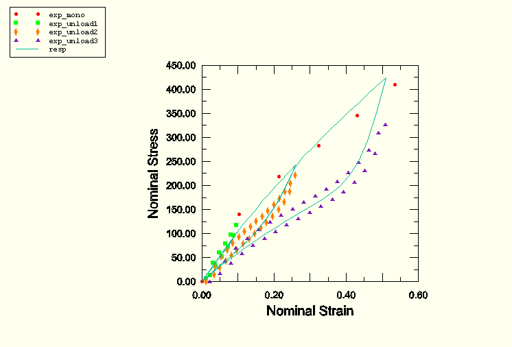
Figure 3.1.7–2 shows the calibrated response of ABAQUS along with the test data. The continuous bold line represents the numerical response for cyclic loading and unloading to the three maximum strain levels for which test data have been provided (the response at the lowest maximum strain level is not visible in the scale of this figure due to a relatively small amount of damage). As the figure illustrates, the model in ABAQUS approximates the stabilized cycle at each strain level with a single curve. The figure also illustrates that the model does not capture the progressive damage during the first few cycles at any strain level. Thus, while the numerical results for unloading from a given strain level begin from the primary curve, the maximum stress for the test results for the stabilized cycle may be somewhat below the measured primary material behavior.

It may be noted that the numerical response can be obtained by carrying out a uniaxial loading/unloading test with a single element. Alternatively, the numerical response for both the primary and the unloading-reloading behavior can be obtained by using the *PREPRINT option with MODEL=YES and simply carrying out a datacheck run. In the latter case the response computed by ABAQUS is printed to the data (.dat) file along with the experimental data. These tabular data can be plotted in ABAQUS/CAE for comparison and evaluation purposes. The primary material behavior can also be evaluated with the automated material evaluation tools available in ABAQUS/CAE.

A solid disc made out of the rubber material described in the earlier section is subjected to cyclic deformation. The coefficients for the Yeoh model determined during the calibration are used along with a value of 5.E–06 to introduce a small amount of compressibility in the material. This value of is obtained based on the measured value of the initial bulk modulus of the rubber. The Mullins effect model in ABAQUS assumes that the damage is associated with the deviatoric behavior only. The disc has an outer diameter of 3 inches, an inner diameter of 1.75 inches, and a thickness of 0.7 inches. The inner surface of the disc is fully constrained. The outer surface is initially defined to be just touching a flat rigid surface. The coefficient of friction between the disc and the rigid surface is assumed to be zero. During the analysis the rigid surface is pushed up 0.15 inches, brought back to its original position, then again pushed up 0.22 inches before being pushed back to its original position. The above deformation history constitutes two displacement-controlled deformation cycles. The analysis is carried out using both ABAQUS/Standard and ABAQUS/Explicit. An axisymmetric model is created to define the geometry of the disc. Symmetric model generation (*SYMMETRIC MODEL GENERATION) is used to create a three-dimensional disc model using first-order reduced-integration bricks (C3D8R elements) with enhanced hourglass control. The ABAQUS/Explicit model is created by importing the model definition from ABAQUS/Standard. The first step in the ABAQUS/Standard analysis is a do-nothing step, which is used to import the initial state into ABAQUS/Explicit.

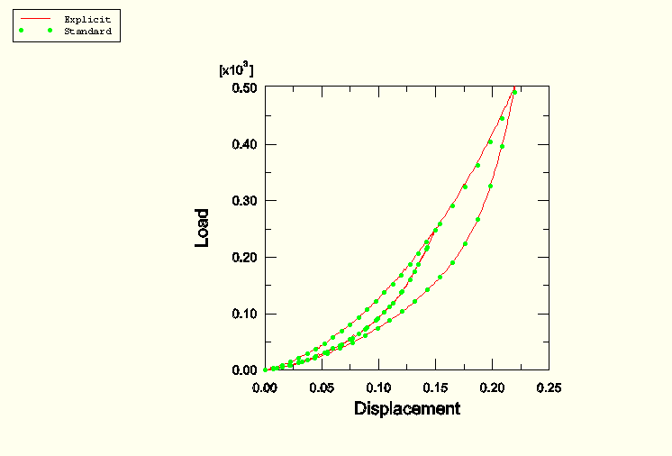
Figure 3.1.7–3 shows the force versus displacement at the rigid body reference node. The two cycles in this figure correspond to the two deformation cycles discussed earlier. During the first cycle the unloading response is softer compared to the loading response due to damage associated with the Mullins effect. During the second loading cycle the response is identical to the unloading segment of the first cycle until the displacement of 0.15 inches is reached. Beyond this point the response is a continuation of the original loading segment of the first cycle. Thus, the load-displacement behavior is consistent with the expected behavior due to the Mullins effect.

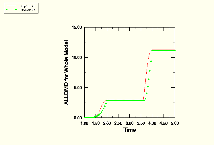
Figure 3.1.7–4 shows the time history of the energy dissipated in the whole model due to damage. The dissipation increases during the loading segment of the first cycle because the material undergoes more and more damage as it is deformed. During the unloading segment of the first cycle and the loading segment of the second cycle up to a displacement of 0.15 inches, no additional damage occurs. As a result, the total dissipation remains constant. For additional displacement beyond 0.15 inches, more damage occurs. This results in further increase of the total damage energy. During the final unloading cycle the damage energy again remains constant.

The loading in the ABAQUS/Explicit analysis is carried out using displacement boundary conditions with an amplitude that uses the smooth step definition (*AMPLITUDE, DEFINITION=SMOOTH STEP) to reduce the noise in the response. Thus, the time history of the displacement is different between the ABAQUS/Standard and the ABAQUS/Explicit simulations, although the total amount of displacement is identical in both analyses. As a result, the time history of the damage dissipation between the two analyses shows some differences in the slope of the response. However, the total dissipation at the end of each stage is identical in the two cases.

The geometry and material of the disc are identical to those described earlier except that the inner surface of the disc is not totally constrained, as it is for the static problem. Instead all the nodes on the inner surface are attached to a node (axle node) located at the center of the disc using kinematic coupling constraints. This facilitates the application of angular velocity or displacement to the axle node to simulate rolling in the Lagrangian approach, as well as the measurement of reaction forces and moments at the axle. The mesh is more refined for the rolling problem compared to the static problem. In particular, two elements are used through the thickness of the disc. The first step is a do-nothing step to facilitate import of the initial state from ABAQUS/Standard to ABAQUS/Explicit. This is followed by a static step in which the rigid surface is pushed against the disc a distance of 0.15 inches. The next step involves rolling of the loaded disc against the rigid surface. This is accomplished in two ways. The first is a Lagrangian analysis in which an angular velocity of 2.5 radians per second is applied to the axle node of the disc. In this example the structure reaches a steady state after one full revolution. No additional damage occurs in subsequent revolution cycles. Therefore, the total time is chosen such that the disc undergoes two revolutions. In the second analysis the rolling is simulated using the steady-state transport (*STEADY STATE TRANSPORT) capability in ABAQUS/Standard. Frictional and inertial effects are neglected in both cases.

The steady-state transport capability directly obtains the steady-state rolling solution of the disc on the rigid surface. Due to Mullins effect the stress state for the rolling solution can be quite different from the stress state for the static non-rolling solution. As a result, an attempt to obtain a steady-state rolling solution directly from a static non-rolling solution may lead to convergence problems in the Newton's scheme that is used to solve the overall nonlinear system of equations. Since the damage and, hence, the discontinuity in state are independent of the angular rolling speed, a time increment cutback during the steady-state transport step does not overcome the convergence difficulties. Such convergence difficulties can be resolved by introducing the damage gradually over an additional steady-state transport step preceding the actual analysis. In this example this is accomplished by following the static loading step with a steady-state transport step with a small rolling angular speed of 0.25 radians per second and with the MULLINS parameter on the *STEADY STATE TRANSPORT option set equal to RAMP. This step is followed by another steady-state transport step at an angular speed of 2.5 radians per second with the MULLINS parameter set equal to STEP, which provides the solution we are interested in obtaining.

A Lagrangian simulation is also carried out in ABAQUS/Explicit. The kinetic energy is monitored to ensure that the problem remains essentially quasi-static. The revolutions of the disc are carried out by applying a rotational displacement (corresponding to two full revolutions) at the axle node using an amplitude with a smooth step definition (*AMPLITUDE, DEFINITION=SMOOTH STEP) to reduce the noise in the response. The compressibility parameter, , is chosen to be 5.E–05, an order of magnitude higher than the actual value, to obtain relatively higher time increments and, thus, a relatively lower run time.

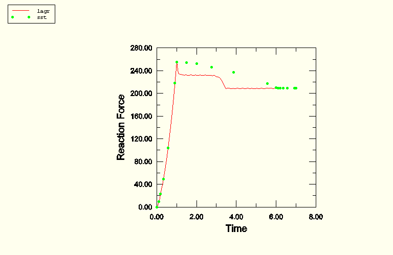
Figure 3.1.7–5 shows a comparison of the time history of the reaction force at the axle node between the Lagrangian and the steady-state rolling analyses in ABAQUS/Standard. The results for the Lagrangian problem (curve labeled lagr) indicate that the reaction force increases during the loading step and decreases during the first revolution of the disc. The decrease in the reaction force is a result of lower overall stresses due to damage in the material. During the second revolution of the disc the reaction force remains constant as no additional damage occurs. The steady-state rolling results (labeled sst) show a gradual transition of the reaction force during the first steady-state transport step that ramps up the Mullins effect. During the second steady-state transport step the reaction force remains constant at the value reached at the end of the prior step. This curve also illustrates that the damage associated with the Mullins effect is independent of the angular speed of rotation. The reaction force remains the same at angular speeds of both 0.25 and 2.5 radians per second. If the Mullins effect is not applied gradually over the first steady-state transport step, the discontinuity between the rolling and the static states may lead to convergence difficulties.

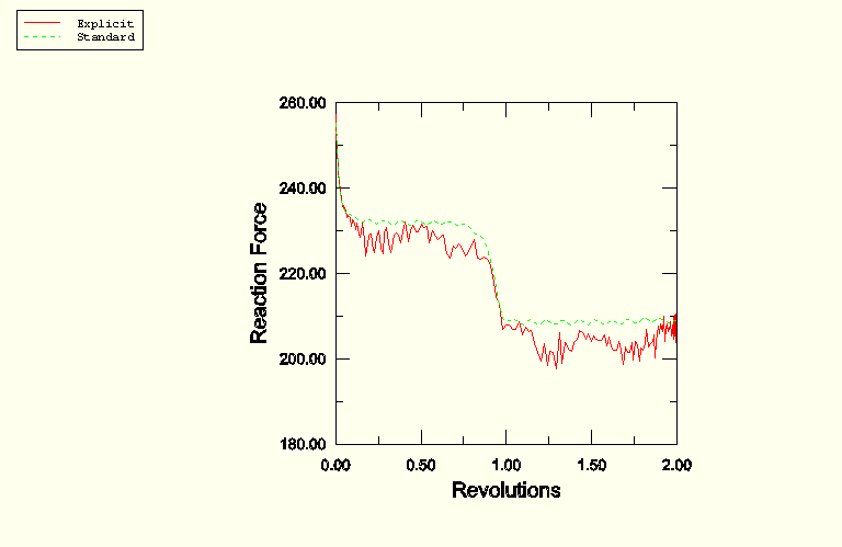
The same results can be observed from a different viewpoint in Figure 3.1.7–6, which shows the reaction force as a function of the number of revolutions for both ABAQUS/Standard and ABAQUS/Explicit. The reaction force decreases during the first revolution and remains steady (except for the noise in the ABAQUS/Explicit analysis) during the second revolution.

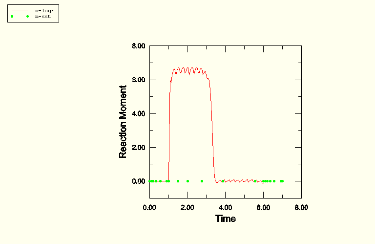
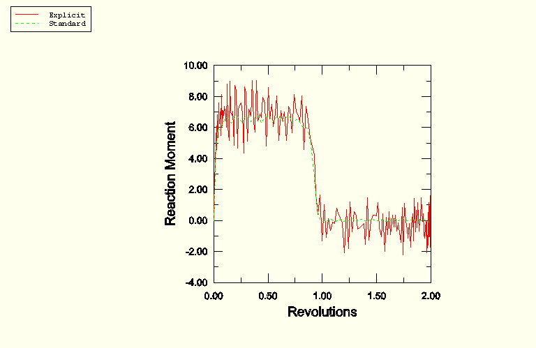
Figure 3.1.7–7 shows a comparison of the time histories of the reaction moment at the axle node between the Lagrangian and the steady-state rolling solutions. The Lagrangian results are labeled m-lagr, while the steady-state rolling results are labeled m-sst. If the material were purely hyperelastic (without damage), the contact forces would be symmetric about a plane normal to the rigid surface and containing the axle; hence, no torque would be required to rotate the disc. However, as a result of the damage associated with Mullins effect the contact forces are not symmetrical as material particles transition through the contact area during the very first revolution. This leads to the reaction moment during the first revolution, as shown in the results for the Lagrangian analysis. The moment reduces to zero during the second revolution. The steady-state rolling results do not include the transient solution of the first revolution; hence, they show a zero moment at all times. Figure 3.1.7–8 shows the same results from a different viewpoint. In this figure the reaction moment is plotted as a function of the number of revolutions for both ABAQUS/Standard and ABAQUS/Explicit.

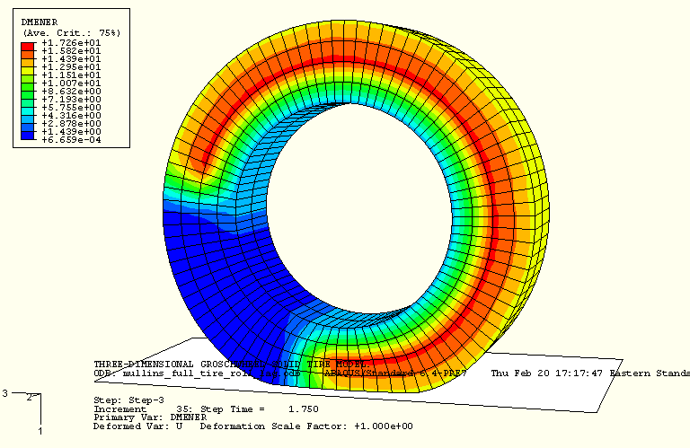
Figure 3.1.7–9 shows a contour plot of the damage energy dissipated at material points at an instant of time that corresponds to about three-quarters of the way into the first revolution of the disc. The figure indicates damage in the material that has already passed through the contact area and no damage in the material that is yet to pass through the contact area. This corresponds to damage in about three-quarters of the disc material. The remaining quarter is still undamaged, as it has not undergone any deformation yet. The full disc will be damaged at the end of the first revolution, and the damage state remains unchanged during the second revolution.