Product: ABAQUS/Explicit
This example illustrates the use of adaptive meshing to model an inviscid fluid sloshing inside a baffled tank. The overall structural response resulting from the coupling between the water and tank, rather than a detailed solution in the fluid, is sought. Adaptive meshing permits the investigation of this response over longer time periods than a pure Lagrangian approach would because the mesh entanglement that occurs in the latter case is prevented.
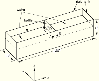
The geometry for the problem is shown in Figure 2.1.14–1. The model consists of a baffled tank filled with water. The baffle, which is attached to the sides and top of the tank, does not penetrate the entire depth of the water. The tank measures 508 × 152.4 × 152.4 mm (20 × 6 × 6 inches), and the baffle measures 3.048 × 152.4 × 121.92 mm (0.12 × 6 × 4.8 inches). The tank is filled with 101.6 mm (4 inches) of water.
A cutaway view of the finite element model that displays the baffle and the water is shown in Figure 2.1.14–2. The top of the tank is not modeled because the water is not expected to come into contact with it. The tank is modeled as a rigid body and is meshed with R3D4 elements. The baffle is modeled as a deformable body and is meshed with S4R elements. A graded mesh of C3D8R elements is used for the water, with more refinement adjacent to the baffle where significant deformations are expected.
In sloshing problems water can be considered an incompressible and inviscid material. An effective method for modeling water in ABAQUS/Explicit is to use a simple Newtonian viscous shear model and a linear ![]() equation of state for the bulk response. The bulk modulus functions as a penalty parameter for the incompressible constraint. Since sloshing problems are unconfined, the bulk modulus chosen can be two or three orders of magnitude less than the actual bulk modulus and the water will still behave as an incompressible medium. The shear viscosity also acts as a penalty parameter to suppress shear modes that could tangle the mesh. The shear viscosity chosen should be small because water is inviscid; a high shear viscosity will result in an overly stiff response. An appropriate value for the shear viscosity can be calculated based on the bulk modulus. To avoid an overly stiff response, the internal forces arising due to the deviatoric response of the material should be kept several orders of magnitude below the forces arising due to the volumetric response. This can be done by choosing an elastic shear modulus that is several orders of magnitude lower than the bulk modulus. If the Newtonian viscous deviatoric model is used, the shear viscosity specified should be on the order of an equivalent shear modulus, calculated as mentioned earlier, scaled by the stable time increment. The expected stable time increment can be obtained from a datacheck analysis of the model. This method is a convenient way to approximate a shear strength that will not introduce excessive viscosity in the material.
equation of state for the bulk response. The bulk modulus functions as a penalty parameter for the incompressible constraint. Since sloshing problems are unconfined, the bulk modulus chosen can be two or three orders of magnitude less than the actual bulk modulus and the water will still behave as an incompressible medium. The shear viscosity also acts as a penalty parameter to suppress shear modes that could tangle the mesh. The shear viscosity chosen should be small because water is inviscid; a high shear viscosity will result in an overly stiff response. An appropriate value for the shear viscosity can be calculated based on the bulk modulus. To avoid an overly stiff response, the internal forces arising due to the deviatoric response of the material should be kept several orders of magnitude below the forces arising due to the volumetric response. This can be done by choosing an elastic shear modulus that is several orders of magnitude lower than the bulk modulus. If the Newtonian viscous deviatoric model is used, the shear viscosity specified should be on the order of an equivalent shear modulus, calculated as mentioned earlier, scaled by the stable time increment. The expected stable time increment can be obtained from a datacheck analysis of the model. This method is a convenient way to approximate a shear strength that will not introduce excessive viscosity in the material.
In addition, if a shear model is defined, the hourglass control forces are calculated based on the shear stiffness of the material. Thus, in materials with extremely low or zero shear strengths such as inviscid fluids, the hourglass forces calculated based on the default parameters are insufficient to prevent spurious hourglass modes. Therefore, a sufficiently high hourglass scaling factor is used to increase the resistance to such modes. This analysis methodology is verified in “Water sloshing in a pitching tank,” Section 1.11.7 of the ABAQUS Benchmarks Manual.
For this example the linear ![]() equation of state is used with a wave speed of 45.85 m/sec (1805 in/sec) and a density of 983.204 kg/m3 (0.92 × 10⁻⁴ lb sec2/in4). The wave speed corresponds to a bulk modulus of 2.07 MPa (300 psi), three orders of magnitude less than the actual bulk modulus of water, 2.07 GPa (3.0 × 10⁵ psi). The shear viscosity is chosen as 1.5 × 10⁻⁸ psi sec. The baffle is modeled as a Mooney-Rivlin elastomeric material with hyperelastic constants
equation of state is used with a wave speed of 45.85 m/sec (1805 in/sec) and a density of 983.204 kg/m3 (0.92 × 10⁻⁴ lb sec2/in4). The wave speed corresponds to a bulk modulus of 2.07 MPa (300 psi), three orders of magnitude less than the actual bulk modulus of water, 2.07 GPa (3.0 × 10⁵ psi). The shear viscosity is chosen as 1.5 × 10⁻⁸ psi sec. The baffle is modeled as a Mooney-Rivlin elastomeric material with hyperelastic constants ![]() = 689480 Pa (100 psi) and
= 689480 Pa (100 psi) and ![]() = 172370 Pa (25 psi) and a density of 10900.74 kg/m3 (1.02 × 10⁻³ lb sec2/in4).
= 172370 Pa (25 psi) and a density of 10900.74 kg/m3 (1.02 × 10⁻³ lb sec2/in4).
Pure master-slave contact is defined between the tank and the water; balanced master-slave contact is defined between the baffle and the water. The bottom edge of the baffle has nodes in common with the underlying water surface. This prevents relative slip between the bottom edge of the baffle and the water immediately below it. The motion of the other edges of the baffle coincides with that of the tank.
The water is subjected to gravity loading. Consequently, an initial geostatic stress field is defined to equilibrate the stresses caused by the self-weight of the water. A velocity pulse in the form of a sine wave with an amplitude of 63.5 mm (2.5 inches) and a period of 2 seconds is prescribed for the tank in both the x- and y-directions simultaneously. All remaining degrees of freedom for the tank are fully constrained. The sloshing analysis is performed for two seconds.
A single adaptive mesh domain that incorporates the water is defined. Sliding boundary regions are used for all contact surface definitions on the water (the default). Because the sloshing phenomenon modeled in this example results in large mesh motions, it is necessary to increase the frequency and intensity of adaptive meshing. The frequency value is reduced to 5 increments from a default value of 10, and the number of mesh sweeps used to smooth the mesh is increased to 3 from a default value of 1. The SMOOTHING OBJECTIVE parameter on the *ADAPTIVE MESH CONTROLS option is set to GRADED so that the initial mesh gradation of the water is preserved while continuous adaptive meshing is performed. The default values are used for all other parameters and controls.
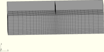
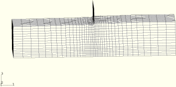
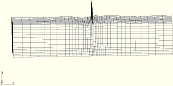
Figure 2.1.14–3, Figure 2.1.14–4, and Figure 2.1.14–5 show the deformed mesh configuration at ![]() 1.2 s,
1.2 s, ![]() 1.6 s, and
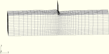
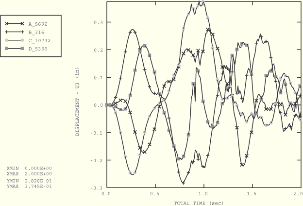
1.6 s, and ![]() 2.0 s, respectively. Four time histories of the vertical displacement of the water level are shown in Figure 2.1.14–6; these correspond to the water level at the baffle in the front and back of the left and right bays. The locations at which the time histories are measured are denoted A, B, C, and D in Figure 2.1.14–1. An analysis such as this could be used to design a baffle that attenuates sloshing at certain frequencies. Using adaptivity in ABAQUS/Explicit is appropriate for sloshing problems in which the structural response is of primary interest. It is generally not possible to model such flow behaviors as splashing or complex free surface interactions. Furthermore, surface tension is not modeled.
2.0 s, respectively. Four time histories of the vertical displacement of the water level are shown in Figure 2.1.14–6; these correspond to the water level at the baffle in the front and back of the left and right bays. The locations at which the time histories are measured are denoted A, B, C, and D in Figure 2.1.14–1. An analysis such as this could be used to design a baffle that attenuates sloshing at certain frequencies. Using adaptivity in ABAQUS/Explicit is appropriate for sloshing problems in which the structural response is of primary interest. It is generally not possible to model such flow behaviors as splashing or complex free surface interactions. Furthermore, surface tension is not modeled.