Product: ABAQUS/Explicit
This example simulates a high velocity, oblique impact of a copper rod into a rigid wall. Extremely high plastic strains develop at the crushed end of the rod, resulting in severe local mesh distortion. Adaptive meshing is used to reduce element distortion and to obtain an accurate and economical solution to the problem.
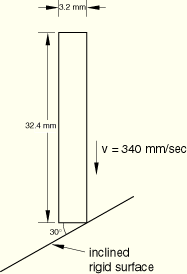
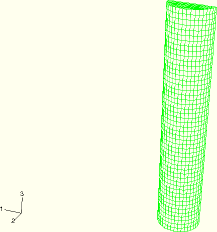
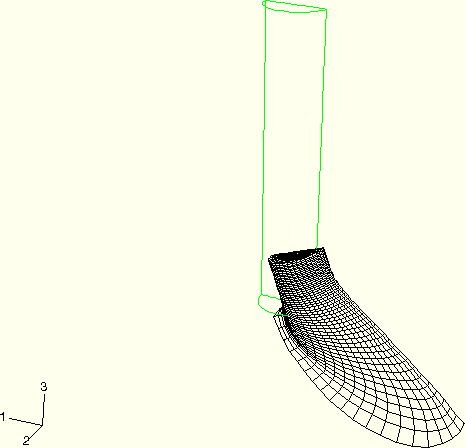
The model geometry is depicted in Figure 2.1.13–1. A cylindrical rod, measuring 32.4 × 3.2 mm, impacts a rigid wall with an initial velocity of ![]() =340 m/sec. The wall is perpendicular to the x–z plane and makes an angle of 30° with the x–y plane. The half-symmetric finite element model is shown in Figure 2.1.13–2. Symmetry boundary conditions are applied at the y=0 plane. The rod is meshed with CAX4R elements, and the wall is modeled as an analytical rigid surface using the *SURFACE, TYPE=CYLINDER option in conjunction with the *RIGID BODY option. Coulomb friction is assumed between the rod and the wall, with a friction coefficient of 0.2. The analysis is performed for a period of 120 microseconds.
=340 m/sec. The wall is perpendicular to the x–z plane and makes an angle of 30° with the x–y plane. The half-symmetric finite element model is shown in Figure 2.1.13–2. Symmetry boundary conditions are applied at the y=0 plane. The rod is meshed with CAX4R elements, and the wall is modeled as an analytical rigid surface using the *SURFACE, TYPE=CYLINDER option in conjunction with the *RIGID BODY option. Coulomb friction is assumed between the rod and the wall, with a friction coefficient of 0.2. The analysis is performed for a period of 120 microseconds.
The rod is modeled as a Johnson-Cook, elastic-plastic material with a Young's modulus of 124 GPa, a Poisson's ratio of 0.34, and a density of 8960 kg/m3. The Johnson-Cook model is appropriate for modeling high-rate impacts involving metals. The Johnson-Cook material parameters are taken from Johnson and Cook (1985) in which the following constants are used: ![]() 90 MPa,
90 MPa, ![]() 0.31,
0.31, ![]() 1.09,
1.09, ![]() 0.025, and
0.025, and ![]() 1 s–1. Furthermore, the melting temperature is 1058°C, and the transition temperature is 25°C. Adiabatic conditions are assumed with a heat fraction of 50%. The specific heat of the material is 383 J/Kg°C, and the thermal expansion coefficient is 0.00005°C–1.
1 s–1. Furthermore, the melting temperature is 1058°C, and the transition temperature is 25°C. Adiabatic conditions are assumed with a heat fraction of 50%. The specific heat of the material is 383 J/Kg°C, and the thermal expansion coefficient is 0.00005°C–1.
A single adaptive mesh domain that incorporates the entire rod is defined. Symmetry boundary conditions are defined as Lagrangian surfaces (the default), and contact surfaces are defined as sliding contact surfaces (the default). Because the impact phenomenon modeled in this example is an extremely dynamic event with large changes in geometry occurring over a relatively small number of increments, it is necessary to increase the frequency and intensity of adaptive meshing. The frequency value is reduced to 5 increments from a default value of 10, and the number of mesh sweeps used to smooth the mesh is increased to 3 from the default value of 1. The default values are used for all other adaptive mesh controls.
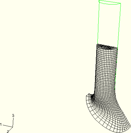
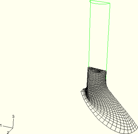
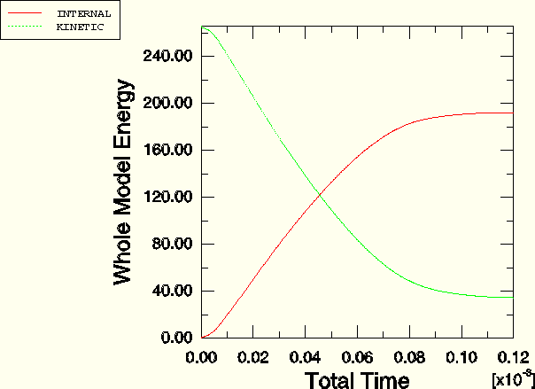
Deformed shape plots at 40, 80, and 120 microseconds are shown in Figure 2.1.13–3, Figure 2.1.13–4, and Figure 2.1.13–5, respectively. The rod rebounds from the wall near the end of the analysis. High-speed collisions such as these result in significant amounts of material flow in the impact zone. A pure Lagrangian analysis of this finite element model fails as a result of excessive distortions. Continuous adaptive meshing allows the analysis to run to completion while retaining a high-quality mesh. The kinetic and internal energy histories are plotted in Figure 2.1.13–6. Most of the initial kinetic energy is converted to internal energy as the rod is plastically deformed. Both energy curves plateau as the rod rebounds from the wall.
Analysis using adaptive meshing.
External file referenced by this analysis.
Johnson, G. R., and W. H. Cook, “Fracture Characteristics of Three Metals Subjected to Various Strains, Strain Rates, Temperatures and Pressures,” Engineering Fracture Mechanics, 21, pp. 31–48, 1985.