Products: ABAQUS/Standard ABAQUS/Explicit
ABAQUS provides a capability for introducing generalized forces on acoustic and solid media associated with the arrival of dilatational waves. This capability applies to acoustic scattering problems and problems involving blast loads in air or water. Thus, the capability is available in transient dynamic procedures in ABAQUS/Standard and ABAQUS/Explicit.
Consider a dynamic problem involving fluid and coupled solid domains, excited by a propagating wave in the fluid arriving from outside these domains. When the mechanics of a fluid can be described as linear, wave fields in the fluid can be superimposed. Therefore, the observed total pressure in the fluid can be decomposed into two components: the incident wave itself, which is known, and the wave field excited in the fluid due to reflections at the fluid boundaries and interactions with the solid. To compute the latter, “scattered” solution, it is sufficient to apply loads at the boundaries of the fluid and solid domains corresponding to the effects of the incident wave field.
The fluid mechanical behavior is nonlinear when the fluid is capable of undergoing cavitation. In that case superposition of the incident wave and the response due to the boundaries, the solid, and the cavitating fluid regions to the incident wave loading is not valid. A total wave formulation (see “Coupled acoustic-structural medium analysis,” Section 2.9.1) is used in ABAQUS/Explicit to handle the incident wave loads on an acoustic medium capable of undergoing cavitation. In the total wave formulation the incident wave loading is applied as traction on the boundary of the modeled acoustic domain as the wave impinges on this domain from an external source. The default scattered wave formulation applicable in the absence of cavitation is presented below.
The equations for coupled fluid-solid interaction in ABAQUS are developed in “Coupled acoustic-structural medium analysis,” Section 2.9.1. Here, we proceed from the coupled system:
These equations couple the total pressure in the fluid to the displacements in the solid. They are valid for any combination of fluid and solid domains in a particular model: the matrixTo proceed, we decompose the total pressure into the known incident wave component and the unknown scattered component:
![]()
The incident field is independent of the scattered field by convention. Therefore, it can be shown that it is a solution to the equation
![]()
The scattered fluid traction, ![]() , depends on the incident pressure through the decomposition above and the solid motion at the boundary. In the absence of an impedance condition at this boundary, this results in the relation
, depends on the incident pressure through the decomposition above and the solid motion at the boundary. In the absence of an impedance condition at this boundary, this results in the relation
The “virtual mass approximation” is a simplification of the general scattered-field form of the coupled system Equation 6.3.1–1. Physically, it corresponds to considering the fluid wave speed to be very large compared to the characteristic structural wave speeds of interest; that is, fluid disturbances propagate and distribute in the field at an extremely high rate compared to the disturbances in the structure. This can be modeled by imposing an incompressibility condition on the fluid. Formally, applying such a condition results in the suppression of the terms related to time derivatives, volumetric drag, and impedance in the fluid equation for the coupled system:
The fluid will also be assumed to have homogeneous mass density,The matrix operator ![]() is the discrete form of the integral over the wetted or loaded surface (see “Coupled acoustic-structural medium analysis,” Section 2.9.1). If the structure is long and thin, it is often modeled with beam elements. Then it is appropriate to replace the surface integral that generates the
is the discrete form of the integral over the wetted or loaded surface (see “Coupled acoustic-structural medium analysis,” Section 2.9.1). If the structure is long and thin, it is often modeled with beam elements. Then it is appropriate to replace the surface integral that generates the ![]() term with a more convenient volume integral term. Since
term with a more convenient volume integral term. Since
The incident field in the fluid is assumed known; moreover, it is assumed to be associated with a separable solution to the scalar wave equation of the form
![]()
An incident wave produces a time-varying pressure at a spatial point of interest ![]() of the form
of the form
![]()
![]()
![]()
![]()
![]()
The incident wave boundary tractions in the solid equation Equation 6.3.1–4 result from direct substitution of Equation 6.3.1–17. The fluid boundary tractions Equation 6.3.1–4 and the tractions in Equation 6.3.1–15 require the evaluation of the gradient of the incident wave pressure:

![]()
![]()
![]()
![]()
![]()
![]()
Generally, the effects of the motion of the source point, ![]() , are included in the defined amplitude
, are included in the defined amplitude ![]() of the incident wave field (specified at the standoff point
of the incident wave field (specified at the standoff point ![]() ). That is, it is assumed that the stated amplitude reflects the time history at a specific fixed standoff point, including the effects of the source point motion, if any. For example, in underwater shock loading the incident wave field is produced by a pulsating gas bubble, which migrates toward the free surface of the water. Therefore, the corresponding incident wave amplitude model for this effect includes a moving source point.
). That is, it is assumed that the stated amplitude reflects the time history at a specific fixed standoff point, including the effects of the source point motion, if any. For example, in underwater shock loading the incident wave field is produced by a pulsating gas bubble, which migrates toward the free surface of the water. Therefore, the corresponding incident wave amplitude model for this effect includes a moving source point.
The structural model affected by the incident wave may be in motion, as well. For example, a ship can move with respect to an explosive charge source during the loading. Because the wave motion is usually extremely fast compared to the ship motion and because incident wave pulse durations are typically short, some approximations apply. First, it can be assumed that the motion of the standoff point, ![]() , can be described by its position at time zero and by the average velocity during the incident wave loading,
, can be described by its position at time zero and by the average velocity during the incident wave loading, ![]() . In addition, the magnitude of this velocity can be assumed small compared to the speed of wave propagation, so the wave equation itself is unaffected by the relative motion. Furthermore, it can be assumed that the specified amplitude history,
. In addition, the magnitude of this velocity can be assumed small compared to the speed of wave propagation, so the wave equation itself is unaffected by the relative motion. Furthermore, it can be assumed that the specified amplitude history, ![]() , corresponds to observations made at the position of the standoff point at time zero,
, corresponds to observations made at the position of the standoff point at time zero, ![]() .
.
Under these assumptions the effect of structural motion during incident wave loading can be modeled in a reference frame fixed with the standoff point, so the source point appears to move with ![]() :
:
![]()
![]()
An underwater explosion can lead to the formation of a highly compressed bubble that propels the surrounding water radially outward, generating an outward-propagating shockwave. As the bubble expands, the pressure inside decreases until it is considerably below the ambient pressure. After reaching a maximum radius with a minimum pressure, the bubble begins to contract. The contraction proceeds until the bubble collapses to a minimum radius. Because of a large pressure generated inside the bubble during this stage, the bubble begins to expand again, generating a second outward-propagating wave. Once the bubble expands to a second maximum radius, it contracts again. The same expansion-contraction sequence can repeat many times. At the same time during this pulsation process, the bubble migrates upward under the force of buoyancy. As long as the bubble does not reach the free water surface, the expansion-contraction sequence continues, each time with reduced amplitude.
Geers and Hunter (2002) proposed a phenomenological model that treats an underwater explosion as a single bubble event comprised of a shockwave phase and an oscillation phase, with the first phase providing initial conditions to the second.
Based on this model, the volume acceleration during the shockwave phase is given by
in whichIntegration with ![]() and further integration with
and further integration with ![]() then yields
then yields

![]()
These expressions are evaluated at ![]() to determine the initial conditions for the subsequent bubble response calculations during the oscillation phase. This choice was validated since, for a single set of charge constants, the initial condition values for values of
to determine the initial conditions for the subsequent bubble response calculations during the oscillation phase. This choice was validated since, for a single set of charge constants, the initial condition values for values of ![]() between
between ![]() and
and ![]() produce essentially the same response during the oscillation phase, as demonstrated by Geers and Hunter (2002).
produce essentially the same response during the oscillation phase, as demonstrated by Geers and Hunter (2002).
The following are the equations of motion for the doubly asymptotic approximation model to describe the evolution of the bubble radius, ![]() , and migration,
, and migration, ![]() , during the oscillation phase:
, during the oscillation phase:


Seven initial conditions are needed. The first two are ![]() ,
, ![]() , the second two are
, the second two are ![]() ,
, ![]() , the fifth one is
, the fifth one is ![]() , and the remaining two are determined as
, and the remaining two are determined as
![]()
![]()
![]()
The incident pressure induced during the bubble response can be expressed as
wherewith![]()
![]()
Since the constants ![]() and
and ![]() are both substantially smaller than one,
are both substantially smaller than one, ![]() for the shockwave phase above is only weakly dependent on
for the shockwave phase above is only weakly dependent on ![]() . Thus, for simplicity,
. Thus, for simplicity, ![]() can be treated as a constant when the gradient of the pressure is evaluated. In this way all formulations in the previous two sections can be still used without losing any significant accuracy.
can be treated as a constant when the gradient of the pressure is evaluated. In this way all formulations in the previous two sections can be still used without losing any significant accuracy.
The model of Geers and Hunter (2002) can be simplified to ignore the energy losses due to waves in the fluid and the gases. This “waveless” form of the equations more closely reproduces the results of earlier research on this phenomenon.
In the waveless model the shockwave phase of the loading is unchanged from the previous case. The equations of motion for the evolution of the bubble radius and migration during the oscillation phase are simplified, however, using the assumptions
![]()
![]()
![]()
![]()
![]()
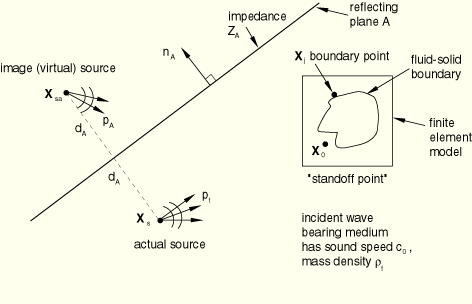
ABAQUS allows the user to specify planes outside the computational domain that reflect the incident wave. This reflected wave is superposed, with a suitable time delay or phase shift, onto the wave arriving at the standoff point via the direct path, forming the total incident wave field for that source. This functionality is implemented for spherical or planar waves and reflection planes at any orientation, which may have arbitrary impedance properties. Only a single reflection from each plane is considered. However, multiple reflections inside the finite element computational domain are considered automatically.
Consider the schematic arrangement of source point, standoff point, and reflection plane ![]() as shown in Figure 6.3.1–1.
as shown in Figure 6.3.1–1.
The actual source is given by
![]()
![]()
![]()
![]()
![]()

![]()
![]()
![]()
In ABAQUS the effects of fluid volumetric drag, the spreading loss due to the distance to the reflection plane, and the complex part of the admittance ![]() are ignored, so the amplitude of the reflected wave is related to the amplitude of the incident wave by
are ignored, so the amplitude of the reflected wave is related to the amplitude of the incident wave by

![]()
![]()
![]()
If a reflecting plane is considered “soft,” the pressure is zero there. Then ![]() and
and
![]()
![]()
The schematic for reflected plane waves is similar to that for spherical waves, except for the geometry of the reflection. In contrast to the spherical case, when planar waves reflect from a boundary (see Figure 6.3.1–2), the direction of the reflected wave is common for all points on the wavefront. The location of the perceived source of the reflected wave is different, however. To calculate the phase shift for the reflected wave incident at an arbitrary point ![]() correctly, the locations of these perceived sources need to be calculated.
correctly, the locations of these perceived sources need to be calculated.
The reflected plane wave load can be calculated on the basis of the reflected wave direction and the time delay associated with the additional path length of the reflected wave. Referring to Figure 6.3.1–2, we see that the reflected wave direction is given by
![]()
![]()
![]()
![]()
![]()
![]()
![]()