Products: ABAQUS/Standard ABAQUS/Explicit
ABAQUS provides a set of elements for modeling a fluid medium undergoing small pressure variations and interface conditions to couple these acoustic elements to a structural model. These elements are provided to model a variety of phenomena involving dynamic interactions between fluid and solid media.
Steady-state harmonic (linear) response analysis can be performed for a coupled acoustic-structural system, such as the study of the noise level in a vehicle. The steady-state procedure is based on direct solution of the coupled complex harmonic equations, as described in “Direct steady-state dynamic analysis,” Section 2.6.1; on a modal-based procedure, as described in “Steady-state linear dynamic analysis,” Section 2.5.7; or on a subspace-based procedure, as described in “Subspace-based steady-state dynamic analysis,” Section 2.6.2. Mode-based linear transient dynamic analysis is also available, as described in “Modal dynamic analysis,” Section 2.5.5.
The acoustic fluid elements can also be used with nonlinear response analysis (implicit or explicit direct integration) procedures: whether such results are useful depends on the applicability of the small pressure change assumption in the fluid. Often, in coupled fluid-solid problems the fluid forces in this linear regime are high enough that nonlinear response of the structure needs to be considered. For example, a ship subjected to underwater incident wave loads due to an explosion may experience plastic deformation, or large motions of internal machinery may occur.
The acoustic medium in ABAQUS may have velocity-dependent dissipation, caused by fluid viscosity or by flow within a resistive porous matrix material. In addition, rather general boundary conditions are provided for the acoustic medium, including impedance, or “reactive,” boundaries.
The possible conditions at the surface of the acoustic medium are:
Prescribed pressure (degree of freedom 8) at the boundary nodes. (Boundary conditions can be used to specify pressure at any node in the model.)
Prescribed inward normal derivative of pressure per unit density of the acoustic medium through the use of a concentrated load on degree of freedom 8 of a boundary node. If the applied load has zero magnitude (that is, if no concentrated load or other boundary condition is present), the inward normal derivative of pressure (and normal fluid particle acceleration) is zero, which means that the default boundary condition of the acoustic medium is a rigid, fixed wall (Neumann condition).
Acoustic-structural coupling defined either by using surface-based coupling procedures (see “Surface-based acoustic-structural medium interaction,” Section 5.2.7) or by placing ASI coupling elements on the interface between the acoustic medium and a structure.
An impedance condition, representing an absorbing boundary between the acoustic medium and a rigid wall or a vibrating structure or representing radiation to an infinite exterior.
An incident wave loading, representing the inward normal derivative of pressure per unit density of the acoustic medium resulting from the arrival of a specified wave. The formulation of this loading case is discussed in “Loading due to an incident dilatational wave field,” Section 6.3.1. It is applicable to problems involving blast loads and to acoustic scattering problems.
The equilibrium equation for small motions of a compressible, adiabatic fluid with velocity-dependent momentum losses is taken to be
whereThe constitutive behavior of the fluid is assumed to be inviscid, linear, and compressible, so
whereFor an acoustic medium capable of undergoing cavitation, the absolute pressure (sum of the static pressure and the excess dynamic pressure) cannot drop below the specified cavitation limit. When the absolute pressure drops to this limit value, the fluid is assumed to undergo free expansion without a corresponding drop in the dynamic pressure. The pressure would rebuild in the acoustic medium once the free expansion that took place during the cavitation is reversed sufficiently to reduce the volumetric strain to the level at the cavitation limit. The constitutive behavior for an acoustic medium capable of undergoing cavitation can be stated as
![]()
![]()
Acoustic fields are strongly dependent on the conditions at the boundary of the acoustic medium. The boundary of a region of acoustic medium that obeys Equation 2.9.1–1 and Equation 2.9.1–2 can be divided into subregions ![]() on which the following conditions are imposed:
on which the following conditions are imposed:
![]() , where the value of the acoustic pressure
, where the value of the acoustic pressure ![]() is prescribed.
is prescribed.
![]() , where we prescribe the normal derivative of the acoustic medium. This condition also prescribes the motion of the fluid particles and can be used to model acoustic sources, rigid walls (baffles), incident wave fields, and symmetry planes.
, where we prescribe the normal derivative of the acoustic medium. This condition also prescribes the motion of the fluid particles and can be used to model acoustic sources, rigid walls (baffles), incident wave fields, and symmetry planes.
![]() , the “reactive” acoustic boundary, where there is a prescribed linear relationship between the fluid acoustic pressure and its normal derivative. Quite a few physical effects can be modeled in this manner: in particular, the effect of thin layers of material, whose own motions are unimportant, placed between acoustic media and rigid baffles. An example is the carpet glued to the floor of a room or car interior that absorbs and reflects acoustic waves. This thin layer of material provides a “reactive surface,” or impedance boundary condition, to the acoustic medium. This type of boundary condition is also referred to as an imposed impedance, admittance, or a “Dirichlet to Neumann map.”
, the “reactive” acoustic boundary, where there is a prescribed linear relationship between the fluid acoustic pressure and its normal derivative. Quite a few physical effects can be modeled in this manner: in particular, the effect of thin layers of material, whose own motions are unimportant, placed between acoustic media and rigid baffles. An example is the carpet glued to the floor of a room or car interior that absorbs and reflects acoustic waves. This thin layer of material provides a “reactive surface,” or impedance boundary condition, to the acoustic medium. This type of boundary condition is also referred to as an imposed impedance, admittance, or a “Dirichlet to Neumann map.”
![]() , the “radiating” acoustic boundary. Often, acoustic media extend sufficiently far from the region of interest that they can be modeled as infinite in extent. In such cases it is convenient to truncate the computational region and apply a boundary condition to simulate waves passing exclusively outward from the computational region.
, the “radiating” acoustic boundary. Often, acoustic media extend sufficiently far from the region of interest that they can be modeled as infinite in extent. In such cases it is convenient to truncate the computational region and apply a boundary condition to simulate waves passing exclusively outward from the computational region.
![]() , where the motion of an acoustic medium is directly coupled to the motion of a solid. On such an acoustic-structural boundary the acoustic and structural media have the same displacement normal to the boundary, but the tangential motions are uncoupled.
, where the motion of an acoustic medium is directly coupled to the motion of a solid. On such an acoustic-structural boundary the acoustic and structural media have the same displacement normal to the boundary, but the tangential motions are uncoupled.
![]() , an acoustic-structural boundary, where the displacements are linearly coupled but not necessarily identically equal, due to the presence of a compliant or reactive intervening layer. This layer induces an impedance condition between the relative normal velocity between acoustic fluid and solid structure and the acoustic pressure. It is analogous to a spring and dashpot interposed between the fluid and solid particles. As implemented in ABAQUS, an impedance boundary condition surface does not model any mass associated with the reactive lining; if such a mass exists, it should be incorporated into the boundary of the structure.
, an acoustic-structural boundary, where the displacements are linearly coupled but not necessarily identically equal, due to the presence of a compliant or reactive intervening layer. This layer induces an impedance condition between the relative normal velocity between acoustic fluid and solid structure and the acoustic pressure. It is analogous to a spring and dashpot interposed between the fluid and solid particles. As implemented in ABAQUS, an impedance boundary condition surface does not model any mass associated with the reactive lining; if such a mass exists, it should be incorporated into the boundary of the structure.
![]() , a boundary between acoustic fluids of possibly differing material properties. On such an interface, displacement continuity requires that the normal forces per unit mass on the fluid particles be equal. This quantity is the natural boundary traction in ABAQUS, so this condition is enforced automatically during element assembly. This is also true in one-dimensional analysis (i.e., piping or ducts), where the relevant acoustic properties include the cross-sectional areas of the elements. Consequently, fluid-fluid boundaries do not require special treatment in ABAQUS.
, a boundary between acoustic fluids of possibly differing material properties. On such an interface, displacement continuity requires that the normal forces per unit mass on the fluid particles be equal. This quantity is the natural boundary traction in ABAQUS, so this condition is enforced automatically during element assembly. This is also true in one-dimensional analysis (i.e., piping or ducts), where the relevant acoustic properties include the cross-sectional areas of the elements. Consequently, fluid-fluid boundaries do not require special treatment in ABAQUS.
In ABAQUS the finite element formulations are slightly different in direct integration transient and steady-state or modal analyses, primarily with regard to the treatment of the volumetric drag loss parameter and spatial variations of the constitutive parameters. To derive a symmetric system of ordinary differential equations for implicit integration, some approximations are made in the transient case that are not needed in steady state. For linear transient dynamic analysis, the modal procedure can be used and is much more efficient.
To derive the partial differential equation used in direct integration transient analysis, we divide Equation 2.9.1–1 by ![]() , take its gradient with respect to
, take its gradient with respect to ![]() , neglect the gradient of
, neglect the gradient of ![]() , and combine the result with the time derivatives of Equation 2.9.1–2 to obtain the equation of motion for the fluid in terms of the fluid pressure:
, and combine the result with the time derivatives of Equation 2.9.1–2 to obtain the equation of motion for the fluid in terms of the fluid pressure:
An equivalent weak form for the equation of motion, Equation 2.9.1–3, is obtained by introducing an arbitrary variational field, ![]() , and integrating over the fluid:
, and integrating over the fluid:
![]()
Except for the imposed pressure on ![]() , all of the other boundary conditions described above can be formulated in terms of
, all of the other boundary conditions described above can be formulated in terms of ![]() . This term has dimensions of acceleration; in the absence of volumetric drag this boundary traction is equal to the inward acceleration of the particles of the acoustic medium:
. This term has dimensions of acceleration; in the absence of volumetric drag this boundary traction is equal to the inward acceleration of the particles of the acoustic medium:
In direct integration transient dynamics we enforce the acoustic boundary conditions as follows:
On ![]() ,
, ![]() is prescribed and
is prescribed and ![]() .
.
On ![]() , where we prescribe the normal derivative of the acoustic pressure per unit density:
, where we prescribe the normal derivative of the acoustic pressure per unit density:
![]()
On ![]() , the reactive boundary between the acoustic medium and a rigid baffle, we apply a condition that relates the velocity of the acoustic medium to the pressure and rate of change of pressure:
, the reactive boundary between the acoustic medium and a rigid baffle, we apply a condition that relates the velocity of the acoustic medium to the pressure and rate of change of pressure:
On ![]() , the radiating boundary, we apply the radiation boundary condition by specifying the corresponding impedance:
, the radiating boundary, we apply the radiation boundary condition by specifying the corresponding impedance:
![]()
On ![]() , the acoustic-structural interface, we apply the acoustic-structural interface condition by equating displacement of the fluid and solid, which enforces the condition
, the acoustic-structural interface, we apply the acoustic-structural interface condition by equating displacement of the fluid and solid, which enforces the condition
![]()
![]()
![]()
![]()
On ![]() , the mixed impedance boundary and acoustic-structural boundary, we apply a condition that relates the relative outward velocity between the acoustic medium and the structure to the pressure and rate of change of pressure:
, the mixed impedance boundary and acoustic-structural boundary, we apply a condition that relates the relative outward velocity between the acoustic medium and the structure to the pressure and rate of change of pressure:
These definitions for the boundary term, ![]() , are introduced into Equation 2.9.1–6 to give the final variational statement for the acoustic medium (this is the equivalent of the virtual work statement for the structure):
, are introduced into Equation 2.9.1–6 to give the final variational statement for the acoustic medium (this is the equivalent of the virtual work statement for the structure):
![]()
![]()
![]()
![]()
Equation 2.9.1–14 and Equation 2.9.1–15 define the variational problem for the coupled fields ![]() and
and ![]() . The problem is discretized by introducing interpolation functions: in the fluid
. The problem is discretized by introducing interpolation functions: in the fluid ![]() ,
, ![]() up to the number of pressure nodes and in the structure
up to the number of pressure nodes and in the structure ![]() ,
, ![]() up to the number of displacement degrees of freedom. In these and the following equations we assume summation over the superscripts that refer to the degrees of freedom of the discretized model. We also use the superscripts
up to the number of displacement degrees of freedom. In these and the following equations we assume summation over the superscripts that refer to the degrees of freedom of the discretized model. We also use the superscripts ![]() ,
, ![]() to refer to pressure degrees of freedom in the fluid and
to refer to pressure degrees of freedom in the fluid and ![]() ,
, ![]() to refer to displacement degrees of freedom in the structure. We use a Galerkin method for the structural system; the variational field has the same form as the displacement:
to refer to displacement degrees of freedom in the structure. We use a Galerkin method for the structural system; the variational field has the same form as the displacement: ![]() . For the fluid we use
. For the fluid we use ![]() but with the subsequent Petrov-Galerkin substitution
but with the subsequent Petrov-Galerkin substitution

The term ![]() is the nodal right-hand-side term for the acoustical degree of freedom
is the nodal right-hand-side term for the acoustical degree of freedom ![]() , or the applied “force” on this degree of freedom. This term is obtained by integration of the normal derivative of pressure per unit density of the acoustic medium over the surface area tributary to a boundary node.
, or the applied “force” on this degree of freedom. This term is obtained by integration of the normal derivative of pressure per unit density of the acoustic medium over the surface area tributary to a boundary node.
In the case of coupled systems where the forces on the structure due to the fluid—![]() are very small compared to the rest of the structural forces—the system can be solved in a “sequentially coupled” manner. The structural equations can be solved with the
are very small compared to the rest of the structural forces—the system can be solved in a “sequentially coupled” manner. The structural equations can be solved with the ![]() term omitted; i.e., in an analysis without fluid coupling. Subsequently, the fluid equations can be solved, with
term omitted; i.e., in an analysis without fluid coupling. Subsequently, the fluid equations can be solved, with ![]() imposed as a boundary condition. This two-step analysis is less expensive and advantageous for systems such as metal structures in air.
imposed as a boundary condition. This two-step analysis is less expensive and advantageous for systems such as metal structures in air.
The equations are integrated through time using the standard implicit (ABAQUS/Standard) and explicit (ABAQUS/Explicit) dynamic integration options. From the implicit integration operator we obtain relations between the variations of the solution variables (here represented by ![]() ) and their time derivatives:
) and their time derivatives:
![]()

For explicit integration the fluid mass matrix is diagonalized in a manner similar to the treatment of structural mass. The explicit central difference procedure described in “Explicit dynamic analysis,” Section 2.4.5, is applied to the coupled system of equations.
As mentioned above, derivation of symmetric ordinary differential equations in the presence of volumetric drag requires some approximations, in addition to those inherent in any finite element method. First, the spatial gradients of the ratio of volumetric drag to mass density in the fluid are neglected. This may be important in lossy, inhomogeneous acoustic media. Second, to maintain symmetry, the effect of volumetric drag on the fluid-solid boundary terms is neglected. Finally, the effect of volumetric drag on the radiation boundary conditions is approximate. If any of these effects is expected to be significant in an analysis, the user should realize that the results obtained are approximate.
From the discretized equation, Equation 2.9.1–17, neglecting any damping terms and any terms associated with a reactive surface, the eigenvalue problem can be stated as
As stated, this problem cannot be solved in ABAQUS due to the unsymmetric stiffness and mass matrices. Introducing an auxiliary variable,Since the original system of equations, Equation 2.9.1–18, is unsymmetric, there are left- and right-hand-side eigenvectors. It can be shown that the left and right eigenvectors are as follows:
![]()
![]()
The only exception worth a brief discussion is the choice for the calculation of the acoustic participation factors and effective masses, as follows. First, a “rigid body” acoustic mode, ![]() , analogous to the rigid body modes for the structural problem outlined in “Variables associated with the natural modes of a model,” Section 2.5.2, is chosen to be a constant pressure field of unity. A total “acoustic mass” is then defined as
, analogous to the rigid body modes for the structural problem outlined in “Variables associated with the natural modes of a model,” Section 2.5.2, is chosen to be a constant pressure field of unity. A total “acoustic mass” is then defined as ![]() . Left and right acoustic participation factors are defined as
. Left and right acoustic participation factors are defined as
![]()
![]()
![]()
![]()
The direct-solution steady-state dynamic analysis procedure is the preferred solution method for acoustics in ABAQUS if volumetric drag and/or acoustic radiation are significant. If these effects are not significant, the mode-based procedure is preferred because of its efficiency.
All model degrees of freedom and loads are assumed to be varying harmonically at an angular frequency ![]() , so we can write
, so we can write
![]()
![]()
![]()
![]()
The development of the variational statement parallels that for the case of transient dynamics, as though the volumetric drag were absent and the density complex. The variational statement is
![]()
![]()
In steady state the boundary traction is defined as
![]()
On ![]() ,
, ![]() is prescribed, analogous to transient analysis.
is prescribed, analogous to transient analysis.
On ![]() , we prescribe
, we prescribe
![]()
On ![]() , the reactive boundary between the acoustic medium and a rigid baffle, we apply
, the reactive boundary between the acoustic medium and a rigid baffle, we apply
On ![]() , the radiating boundary, we apply the radiation boundary condition impedance in the same form as for the reactive boundary but with the parameters as defined in Equation 2.9.1–38 and Equation 2.9.1–39.
, the radiating boundary, we apply the radiation boundary condition impedance in the same form as for the reactive boundary but with the parameters as defined in Equation 2.9.1–38 and Equation 2.9.1–39.
On ![]() , the acoustic-structural interface, we equate the displacement of the fluid and solid as in the transient case. However, the acoustic boundary traction coupling fluid to solid,
, the acoustic-structural interface, we equate the displacement of the fluid and solid as in the transient case. However, the acoustic boundary traction coupling fluid to solid,
![]()
On ![]() , the mixed impedance boundary and acoustic-structural boundary, the condition
, the mixed impedance boundary and acoustic-structural boundary, the condition
![]()
![]()

The above equation uses the complex density, ![]() . We manipulate it into a form that has real coefficients and an additional time derivative through the relations
. We manipulate it into a form that has real coefficients and an additional time derivative through the relations
![]()
Applying Galerkin's principle, the finite element equations are derived as before. We arrive again at Equation 2.9.1–17 with the same matrices except for the damping and stiffness matrices of the acoustic elements and the surfaces that have imposed impedance conditions, which now appear as

For steady-state harmonic response we assume that the structure undergoes small harmonic vibrations, identified by the prefix ![]() , about a deformed, stressed base state, which is identified by the subscript
, about a deformed, stressed base state, which is identified by the subscript ![]() . Hence, the total stress can be written in the form
. Hence, the total stress can be written in the form
![]()
![]()
To solve the steady-state problem, we assume that the governing equations are satisfied in the base state, and we linearize these equations in terms of the harmonic oscillations. For the internal force vector this yields
![]()

![]()
We assume that the loads and (because of linearity) the response are harmonic, and, hence, we can write
![]()
The medium supporting acoustic waves may be flowing through a porous matrix, such as fiberglass used for sound deadening. In this case the parameter ![]() is the flow resistance, the pressure drop required to force a unit flow through the porous matrix. A propagating plane wave with nominal particle velocity
is the flow resistance, the pressure drop required to force a unit flow through the porous matrix. A propagating plane wave with nominal particle velocity ![]() loses energy at a rate
loses energy at a rate
In steady state this linearized equation can be written in the form of Equation 2.9.1–21, with

If the combined viscosity effects are small,
so we can writeIn steady-state form whereSeveral secondary quantities are useful in acoustic analysis, derived from the fundamental acoustic pressure field variable. In steady-state dynamics the acoustic particle velocity at any field point is
![]()
![]()
Equation 2.9.1–11 (or alternatively Equation 2.9.1–9) can be written in a complex admittance form for steady-state analysis:
where we define The termFor absorption of plane waves in an infinite medium with volumetric drag, the complex impedance can be shown to be
For the impedance-based nonreflective boundary condition in ABAQUS/Standard, the equations above are used to determine the required constants ![]() and
and ![]() . They are a function of frequency if the volumetric drag is nonzero. The small-drag versions of these equations are used in the direct time integration procedures, as in Equation 2.9.1–42.
. They are a function of frequency if the volumetric drag is nonzero. The small-drag versions of these equations are used in the direct time integration procedures, as in Equation 2.9.1–42.
Many acoustic studies involve a vibrating structure in an infinite domain. In these cases we model a layer of the acoustic medium using finite elements, to a thickness of ![]() to a full wavelength, out to a “radiating” boundary surface. We then impose a condition on this surface to allow the acoustic waves to pass through and not reflect back into the computational domain. For radiation boundaries of simple shapes—such as planes, spheres, and the like—simple impedance boundary conditions can represent good approximations to the exact radiation conditions. In particular, we include local algebraic radiation conditions of the form
to a full wavelength, out to a “radiating” boundary surface. We then impose a condition on this surface to allow the acoustic waves to pass through and not reflect back into the computational domain. For radiation boundaries of simple shapes—such as planes, spheres, and the like—simple impedance boundary conditions can represent good approximations to the exact radiation conditions. In particular, we include local algebraic radiation conditions of the form
This expression involves independent coefficients for pressure and its first derivative in time, unlike the transient reactive boundary expression (Equation 2.9.1–10), which includes independent coefficients for the first and second derivatives of pressure only. Consequently, to implement this expression, we define the admittance parameters
and so the boundary traction for the transient radiation boundary condition can be written![]()
The values of the parameters ![]() and
and ![]() vary with the geometry of the boundary of the radiating surface of the acoustic medium. The geometries supported in ABAQUS are summarized in Table 2.9.1–1.
vary with the geometry of the boundary of the radiating surface of the acoustic medium. The geometries supported in ABAQUS are summarized in Table 2.9.1–1.
Table 2.9.1–1 Boundary condition parameters.
| Geometry | ||
|---|---|---|
| Plane | ||
| Circle or circular cylinder | ||
| Ellipse or elliptical cylinder | ||
| Sphere | ||
| Prolate spheroid |
These algebraic boundary conditions are approximations to the exact impedance of a boundary radiating into an infinite exterior. The plane wave condition is the exact impedance for plane waves normally incident to a planar boundary. The spherical condition exactly annihilates the first Legendre mode of a radiating spherical surface; the circular condition is asymptotically correct for the first mode (Bayliss et al., 1982). The elliptical and prolate spheroidal conditions are based on expansions of elliptical and prolate spheroidal wave functions in the low-eccentricity limit (Grote and Keller, 1995); the prolate spheroidal condition exactly annihilates the first term of its expansion, while the elliptical condition is asymptotic.
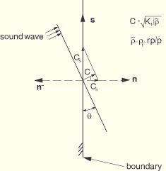
As already pointed out, the radiation boundary conditions derived in the previous section for plane waves are actually based on the presumption that the sound wave impinges on the boundary from an orthogonal direction. But this is not always the case. Figure 2.9.1–1 shows a general example for plane waves in which the sound wave direction differs from the boundary normal by an angle of ![]() .
.
Using the first-order expanding approximation to the second term in the square root in the above equation (similar to what we did to reach Equation 2.9.1–41), we can obtain an improved radiation boundary condition
It can be found from comparison that this equation differs from Equation 2.9.1–42 only by a factor ofThe method described in this section can be used only for direct integration transient dynamics, and it cannot be used with steady-state or modal response. In addition, it is available for planar, axisymmetric, and three-dimensional geometries.
Finally, the method makes the equilibrium equations nonlinear, as shown in Equation 2.9.1–48. Although in theory the iteration process in ABAQUS/Standard can solve the nonlinear equilibrium equations accurately, the use of a small half-step residual tolerance is strongly suggested since in many cases the pressure and its related residual along the radiation boundaries are very weak relative to the other places in the modeled domain. The computation of ![]() at the integration point is based on the nodal pressures. The nodal pressures are updated using the explicit central difference procedure described in “Explicit dynamic analysis,” Section 2.4.5.
at the integration point is based on the nodal pressures. The nodal pressures are updated using the explicit central difference procedure described in “Explicit dynamic analysis,” Section 2.4.5.