The Mullins effect material model provided in ABAQUS is intended for modeling the phenomenon of stress softening, commonly observed in filled rubber elastomers as a result of damage associated with straining. When an elastomeric test specimen is subjected to simple tension from its virgin state, unloaded, and then reloaded, the stress required on reloading is less than that on the initial loading for stretches up to the maximum stretch achieved during the initial loading. This stress-softening phenomenon is known as the Mullins effect (Mullins, 1947).
Material behavior

The following sections describe the Mullins effect model in ABAQUS in detail.
Idealized material behavior
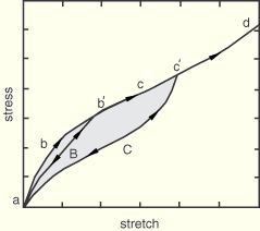
The Mullins effect is depicted qualitatively in Figure 4.7.1–1.
This figure and the accompanying description are based on work by Ogden and Roxburgh (
Ogden and Roxburgh, 1999), which forms the basis of the model implemented in ABAQUS. Consider the primary loading path

of a previously unstressed material, with loading until an arbitrary point

. On unloading from
, the path

is followed. When the material is loaded again, the softened path is retraced as

. If further loading is then applied, the path

is followed, where
is a continuation of the primary loading path

(which is the path that would be followed if there was no unloading). If loading is now stopped at

, the path

is followed on unloading and then retraced back to
on reloading. If no further loading beyond
is applied, the curve

represents the subsequent material response, which is then elastic. For loading beyond
, the primary path is again followed and the pattern described is repeated. This is an ideal representation of Mullins effect. More details regarding the actual behavior and how test data that display such behavior can be used to calibrate the ABAQUS model for Mullins effect are discussed in
“Mullins effect in elastomers,” Section 10.6.1 of the ABAQUS Analysis User's Manual, and in
“Analysis of a solid disc with Mullins effect,” Section 3.1.7 of the ABAQUS Example Problems Manual.
The loading path will henceforth be referred to as the “primary material response,” and the constitutive behavior of the primary response can be defined using the standard energy potentials of the hyperelasticity models in ABAQUS.
Stress softening is interpreted as being due to damage at the microscopic level. As the material is loaded, the damage occurs by the severing of bonds between filler particles and the rubber molecular chains. Different chain links break at different deformation levels, thereby leading to continuous damage with macroscopic deformation. An equivalent interpretation is that the energy required to cause the damage is not recoverable.
Basic framework for the model
Hyperelastic materials are described in terms of a strain energy potential function,  , which defines the strain energy stored in the material per unit reference volume (volume in the initial configuration). The quantity
  may be the deformation gradient tensor or some other appropriate strain measure. To account for Mullins effect, Ogden and Roxburgh proposed a material description that is based on an energy function of the form
  , where
  is a scalar variable. This scalar variable controls the material properties in the sense that it enables the material response to be governed by an energy function on unloading and subsequent submaximal reloading different from that on the primary (initial) loading path from a virgin state. Because of the interpretation and influence of , it is no longer appropriate to think of
  as the stored elastic energy potential. In fact, part of the energy is stored as strain energy, while the rest is dissipated due to damage. The shaded area in Figure 4.7.1–1 represents the energy dissipated by damage, while the unshaded portion represents the recoverable part of the strain energy. As pointed out by Ogden and Roxburgh, the inclusion of results in the following additional equation, due to equilibrium:
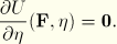
The above equation determines the evolution of
during the course of the deformation. During a deformation process, the variable
may be either active or inactive and may switch from inactive to active or vice versa such that it always varies continously. When it is not active, the material behaves as an elastic material with strain energy
, with
held constant. However, when
is active, it is determined implicitly in terms of
by the preceding equation. The material again behaves as an elastic material but with a different strain energy function

. When the parameter
switches from being active to inactive and vice versa, the energy as well as the associated stresses remain continuous. When
is inactive, it is assumed to have a value of unity without any loss of generality.
Primary hyperelastic behavior
In preparation for writing the constitutive equations for the Mullins effect, it is useful to separate the deviatoric and the volumetric parts of the total strain energy density of the primary material response as
In the above equation
,

, and

are the total, deviatoric, and volumetric parts of the strain energy density, respectively. All the hyperelasticity models in ABAQUS use strain energy potential functions that are already separated into deviatoric and volumetric parts. For example, the polynomial models use a strain energy potential of the form
where the symbols have the usual interpretations. The first term on the right represents the deviatoric part, and the second term represents the volumetric part of the elastic strain energy density function.
Augmented strain energy density function
The Mullins effect is accounted for by using an augmented energy function of the form
where

is the deviatoric part of the strain energy density of the primary material response, defined, for example, by the first term on the right-hand-side of the polynomial strain energy function given above;

is the volumetric part of the strain energy density, defined, for example, by the second term on the right-hand-side of the polynomial strain energy function given above;


represent the deviatoric principal stretches; and

represents the elastic volume ratio. The function

is a continuous function of the damage variable
and is referred to as the “damage function.” As the above expression suggests, the deviatoric part of the augmented energy function is related to the deviatoric part of the energy corresponding to the primary response by the scaling factor
. The volumetric part of the augmented energy function is the same as that for the primary response. A consequence of the above form of the augmented energy function is that the Mullins effect is associated only with the deviatoric part of the deformation. When

, it is required that

, such that

, and the augmented energy function reduces to the strain energy density function of the primary material response. As pointed out earlier, this situation corresponds to
being inactive and physically represents the energy of a material point that is on the primary curve. The value of
varies continuously as the deformation proceeds. The above form of the energy function is an extension of the form proposed by Ogden and Roxburgh to account for material compressibility.
Stress computation
With the above modification to the energy function, the stresses, which are derived from the energy function in the usual manner, are given by
where

is the deviatoric stress corresponding to the primary material response at the current deviatoric deformation level,
, and

is the hydrostatic pressure of the primary material response at the current volumetric deformation level,
. Thus, the deviatoric stress as a result of Mullins effect is obtained by simply scaling the deviatoric stress of the primary material response with the damage variable
. For the above equation to predict stress softening, it is necessary that

on the unloading (and submaximal reloading) path. It is also assumed that

, such that the deviatoric stresses remain positive until

is reached. The pressure stress of the augmented response is the same as that of the primary response. The model predicts unloading-reloading along a single curve (that is different, in general, from the primary loading curve) from any given strain level, that passes through the origin of the stress-strain plot. It cannot capture permanent strains upon removal of load. The model also predicts that a purely volumetric deformation will not have any damage or Mullins effect associated with it.
Damage function and damage variable
As a result of the assumed form of and the evolution equation for , the function satisfies
which implicitly defines the damage parameter
in terms of the deformation as long as the function

is a monotonic function of its argument. The value of
derived from the above equation will depend on the maximum values of the principal stretches

and

attained on a primary loading path and also on the specific forms of the functions

and
used. On the primary curve at any point where the unloading is initiated,

, and the above equation specializes to
which defines the notation

. On the other hand, when the material is fully unloaded with

and
attains its minimum value,

:
From the preceding two equations it follows that both the function
and the quantity
depend on the point

at which unloading is initiated.
When the material is in a fully unloaded state (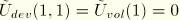 ), the augmented energy function has the residual value
which may be interpreted as the amount of energy dissipated by damage in the material. In a uniaxial test such as simple tension, this quantity denotes the area between the primary loading curve and the relevant unloading-reloading curve (the shaded area in
Figure 4.7.1–1 for deformation until
). Recalling that the function

depends, through

, on the point at which unloading starts, the function
may be constructed, following Ogden and Roxburgh, using
where the function

must satisfy
and
. For a given
, the above equation can be integrated to obtain
as
On the primary path
, and the above equation satisfies the requirement

. ABAQUS uses the following specific choice for

, which has the required properties
The quantities

,

, and

are material constants, and

is the inverse of the error function, where the error function is defined as
The above choice of
reduces to the form proposed by Ogden and Roxburgh when

.
On substituting the above form of in the equation  , it can be shown that the damage variable varies with the deformation according to
The above equation defines the evolution of the damage variable
with deformation

, the maximum value of the deviatoric strain energy density experienced by the material point during its deformation history,
, and material constants
,
, and
. While the parameters
and
are dimensionless, the parameter
has the dimensions of energy.
When  , corresponding to a point on the primary curve,
  . On the other hand,
  attains its minimum value, upon removal of deformation, when
  . For all intermediate values of
  , varies monotonically between and
  .
.
Damage dissipation
As pointed out in the earlier discussion, the quantity  determines the energy dissipated due to damage. The equation for can be integrated analytically through a change of variable of integration from to
  to yield the following expression for the function :
The damage dissipation can be obtained from the above expression by substituting

(with
obtained by setting
in the expression for
) and is given by
The recoverable part of the strain energy,

, can then be obtained by subtracting the damage dissipation from the total augmented energy
When the material is fully or almost incompressible, we may assume that
, and the total energy corresponding to the maximum deformation along the primary curve is given by

The discussion below pertains to the above limit. From the expression for the damage dissipation,
, it may be noted that when

, the ratio of dissipation to
is a constant that depends only on the material parameters
and
. In particular, this ratio is independent of

, suggesting that the ratio of the dissipation to the total energy is a constant that is independent of the level of deformation. For nonzero
the above is true only when

, which correponds to relatively large levels of deformation. In that case when

, the energy dissipation is zero. Thus, the value of
(both zero and nonzero) may be thought of as providing a scale of the strain energy level for the total deformation beyond which dissipation takes place. In particular, when
, dissipation occurs at low strain levels.
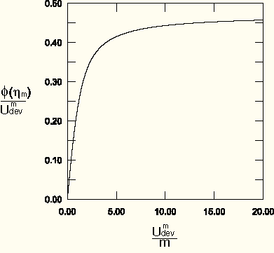
The behavior described above is depicted in Figure 4.7.1–2, which shows a plot of the normalized dissipation,  , versus the ratio
  , for nonzero and for fixed values of the parameters
  and
and  . For small values of the ratio the dissipation tends to zero, while for larger values of the ratio, the normalized dissipation approaches a constant asymptotic value.