Product: ABAQUS/Explicit
This section describes the cracking constitutive model provided in ABAQUS/Explicit for concrete and other brittle materials. The material library in ABAQUS also includes a constitutive model for concrete based on theories of scalar plastic damage, described in “Damaged plasticity model for concrete and other quasi-brittle materials,” Section 4.5.2, which is available in ABAQUS/Standard and ABAQUS/Explicit. In ABAQUS/Standard plain concrete can also be analyzed with the smeared crack concrete model described in “An inelastic constitutive model for concrete,” Section 4.5.1. Although this brittle cracking model can also be useful for other materials, such as ceramics and brittle rocks, it is primarily intended to model plain concrete. Therefore, in the remainder of this section, the physical behavior of concrete is used to motivate the different aspects of the constitutive model.
Reinforced concrete modeling in ABAQUS is accomplished by combining standard elements, using this plain concrete cracking model, with “rebar elements”—rods, defined singly or embedded in oriented surfaces, that use a one-dimensional strain theory and that can be used to model the reinforcing itself. The rebar elements are superposed on the mesh of plain concrete elements and are used with standard metal plasticity models that describe the behavior of the rebar material. This modeling approach allows the concrete behavior to be considered independently of the rebar, so this section discusses the plain concrete cracking model only. Effects associated with the rebar/concrete interface, such as bond slip and dowel action, cannot be considered in this approach except by modifying some aspects of the plain concrete behavior to mimic them (such as the use of “tension stiffening” to simulate load transfer across cracks through the rebar).
It is generally accepted that concrete exhibits two primary modes of behavior: a brittle mode in which microcracks coalesce to form discrete macrocracks representing regions of highly localized deformation, and a ductile mode where microcracks develop more or less uniformly throughout the material, leading to nonlocalized deformation. The brittle behavior is associated with cleavage, shear and mixed mode fracture mechanisms that are observed under tension and tension-compression states of stress. It almost always involves softening of the material. The ductile behavior is associated with distributed microcracking mechanisms that are primarily observed under compression states of stress. It almost always involves hardening of the material, although subsequent softening is possible at low confining pressures. The cracking model described here models only the brittle aspects of concrete behavior. Although this is a major simplification, there are many applications where only the brittle behavior of the concrete is significant; and, therefore, the assumption that the material is linear elastic in compression is justified in those cases.
A smeared model is chosen to represent the discontinuous macrocrack brittle behavior. In this approach we do not track individual “macro” cracks: rather, the presence of cracks enters into the calculations by the way the cracks affect the stress and material stiffness associated with each material calculation point.
Here, for simplicity, the term “crack” is used to mean a direction in which cracking has been detected at the material calculation point in question. The closest physical concept is that there exists a continuum of microcracks at the point, oriented as determined by the model. The anisotropy introduced by cracking is included in the model since it is assumed to be important in the simulations for which the model is intended.
Some objections have been raised against smeared crack models. The principal concern is that this modeling approach inherently introduces mesh sensitivity in the solutions, in the sense that the finite element results do not converge to a unique result. For example, since cracking is associated with strain softening, mesh refinement will lead to narrower crack bands. Many researchers have addressed this concern, and the general consensus is that Hilleborg's (1976) approach—based on brittle fracture concepts—is adequate to deal with this issue for practical purposes. A length scale, typically in the form of a “characteristic” length, is introduced to “regularize” the smeared continuum models and attenuate the sensitivity of the results to mesh density. This aspect of the model is discussed in detail later.
Various researchers have proposed three basic crack direction models (Rots and Blaauwendraad, 1989): fixed, orthogonal cracks; the rotating crack model; and fixed, multidirectional (nonorthogonal) cracks. In the fixed, orthogonal crack model the direction normal to the first crack is aligned with the direction of maximum tensile principal stress at the time of crack initiation. The model has memory of this crack direction, and subsequent cracks at the point under consideration can only form in directions orthogonal to the first crack. In the rotating crack concept only a single crack can form at any point (aligned with the direction of maximum tensile principal stress). Thus, the single crack direction rotates with the direction of the principal stress axes. This model has no memory of crack direction. Finally, the multidirectional crack model allows the formation of any number of cracks at a point as the direction of the principal stress axes changes with loading. In practice, some limitation is imposed on the number of cracks allowed to form at a point. The model has memory of all crack directions.
The multidirectional crack model is the least popular, mainly because the criterion used to decide when subsequent cracks form (to limit the number of cracks at a point) is somewhat arbitrary: the concept of a “threshold angle” is introduced to prevent new cracks from forming at angles less than this threshold value to existing cracks. The fixed orthogonal and rotating crack models have both been used extensively, even though objections can be raised against both. In the rotating crack model the concept of crack closing and reopening is not well-defined because the orientation of the crack can vary continuously. The fixed orthogonal crack model has been criticized mainly because the traditional treatment of “shear retention” employed in the model tends to make the response of the model too stiff. This problem can be resolved by formulating the shear retention in a way that ensures that the shear stresses tend to zero as deformation on the crack interfaces takes place (this is done in the ABAQUS model, as described later). Finally, although the fixed orthogonal crack model has the orthogonality limitation, it is considered superior to the rotating crack model in cases where the effect of multiple cracks is important (the rotating crack model is restricted to a single crack at any point).
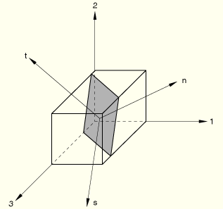
The fixed orthogonal cracks model is used in ABAQUS so that the maximum number of cracks at a material point is limited by the number of direct stress components present at that material point of the finite element model (for example, a maximum of three cracks in three-dimensional, axisymmetric, and plane strain problems or a maximum of two cracks in plane stress problems). Once cracks exist at a point, the component forms of all vector and tensor valued quantities are rotated so that they lie in the local system defined by the crack orientation vectors (the normals to the crack faces). The model ensures that these crack face normal vectors are orthogonal so that this local system is rectangular Cartesian. Crack closing and reopening can take place along the directions of the crack surface normals. The model neglects any permanent strain associated with cracking; that is, we assume that the cracks can close completely when the stress across them becomes compressive.
The main ingredients of the model are a strain rate decomposition into elastic (concrete) and cracking strain rates, elasticity, a set of cracking conditions, and a cracking relation (the evolution law for the cracking behavior). The main advantage of the strain decomposition is that it allows the eventual addition of other effects, such as plasticity and creep, in a consistent manner. The elastic-cracking strain decomposition also allows the separate identification of a cracking strain that represents the state of a crack; this contrasts with the classical smeared cracking models where a single strain quantity is used to represent the state of a cracked solid in a homogenized form leading to a modified (damaged) elasticity formulation.
We begin with a strain rate decomposition,
whereThe strains in Equation 4.5.3–1 are referred to the global Cartesian coordinate system and can be written in vector form (in a three-dimensional setting) as
![]()
![]()
The conjugate stress quantities can be written in the global coordinate system as
![]()
![]()
The intact continuum between the cracks is modeled with isotropic, linear elasticity. The orthotropic nature of the cracked material is introduced in the cracking component of the model. As stated earlier, the approach of decomposing the strains into elastic, intact concrete, strains, and cracking strains has the advantage that this smeared model can be generalized to include other effects such as plasticity and creep (although such generalizations are not yet included in ABAQUS/Explicit).
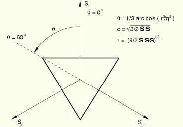
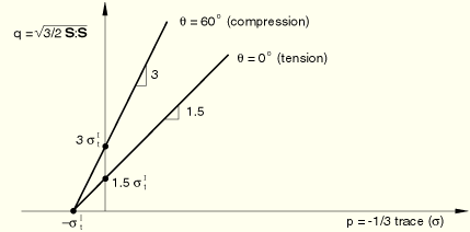
A simple Rankine criterion is used to detect crack initiation. This states that a crack forms when the maximum principal tensile stress exceeds the tensile strength of the brittle material. The Rankine crack detection surface is shown in Figure 4.5.3–2 in the deviatoric plane, in Figure 4.5.3–3 in the meridional plane, and in Figure 4.5.3–4 in plane stress. Although crack detection is based purely on Mode I fracture considerations, ensuing cracked behavior includes both Mode I (tension softening) and Mode II (shear softening/retention) behavior, as described later.
As soon as the Rankine criterion for crack formation has been met, we assume that a first crack has formed. The crack surface is taken to be normal to the direction of the maximum tensile principal stress. Subsequent cracks can form with crack surface normals in the direction of maximum principal tensile stress that is orthogonal to the directions of any existing crack surface normals at the same point.
The crack orientations are stored for subsequent calculations, which are done for convenience in a local coordinate system oriented in the crack directions. Cracking is irrecoverable in the sense that, once a crack has occurred at a point, it remains throughout the rest of the calculation. However, a crack may subsequently close and reopen.
We introduce a consistency condition for cracking (analogous to the yield condition in classical plasticity) written in the crack direction coordinate system in the form of the tensor
where![]()
Each cracking condition is more complex than a classical yield condition in the sense that two cracking states are possible (an actively opening crack state and a closing/reopening crack state), contrasting with a single plastic state in classical plasticity. This can be illustrated by writing the cracking conditions for a particular crack normal direction ![]() explicitly:
explicitly:
![]()
The cracking conditions for the shear components in the crack coordinate system are activated when the associated normal directions are cracked. We now present the shear cracking conditions by writing the conditions for shear component ![]() explicitly.
explicitly.
The crack opening dependent shear model (shear retention model) is written as
for shear loading or unloading of the crack, whereThe relation between the local stresses and the cracking strains at the crack interfaces is written in rate form as
whereUsing the strain rate decomposition (Equation 4.5.3–3) and the elasticity relations, we can write the rate of stress as
wherePremultiplying Equation 4.5.3–9 by ![]() and substituting Equation 4.5.3–5 and Equation 4.5.3–8 into the resulting left-hand side yields
and substituting Equation 4.5.3–5 and Equation 4.5.3–8 into the resulting left-hand side yields
Finally, substituting Equation 4.5.3–10 into Equation 4.5.3–9 results in the stress-strain rate equations:
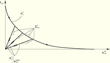
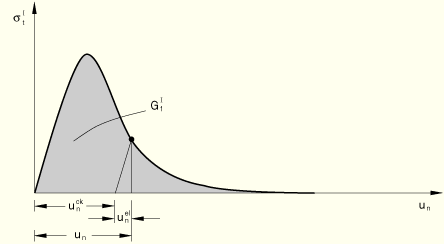
The brittle fracture concept of Hilleborg (1976) forms the basis of the postcracked behavior in the direction normal to the crack surface (commonly referred to as tension softening). We assume that the fracture energy required to form a unit area of crack surface in Mode I, ![]() , is a material property. This value can be calculated from measuring the tensile stress as a function of the crack opening displacement (Figure 4.5.3–7), as
, is a material property. This value can be calculated from measuring the tensile stress as a function of the crack opening displacement (Figure 4.5.3–7), as
![]()
Typical values of ![]() range from 40 N/m (0.22 lb/in) for a typical construction concrete (with a compressive strength of approximately 20 MPa, 2850 lb/in2) to 120 N/m (0.67 lb/in) for a high strength concrete (with a compressive strength of approximately 40 MPa, 5700 lb/in2).
range from 40 N/m (0.22 lb/in) for a typical construction concrete (with a compressive strength of approximately 20 MPa, 2850 lb/in2) to 120 N/m (0.67 lb/in) for a high strength concrete (with a compressive strength of approximately 40 MPa, 5700 lb/in2).
The implication of assuming that ![]() is a material property is that, when the elastic part of the displacement,
is a material property is that, when the elastic part of the displacement, ![]() , is eliminated, the relationship between the stress and the remaining part of the displacement,
, is eliminated, the relationship between the stress and the remaining part of the displacement, ![]() , is fixed, regardless of the specimen size. For example, consider a specimen developing a single crack across its section as tensile displacement is applied to it:
, is fixed, regardless of the specimen size. For example, consider a specimen developing a single crack across its section as tensile displacement is applied to it: ![]() is the displacement across the crack and is not changed by using a longer or shorter specimen in the test (so long as the specimen is significantly longer than the width of the crack band, which will typically be of the order of the aggregate size). Thus, this important part of the cracked concrete's tensile behavior is defined in terms of a stress/displacement relationship.
is the displacement across the crack and is not changed by using a longer or shorter specimen in the test (so long as the specimen is significantly longer than the width of the crack band, which will typically be of the order of the aggregate size). Thus, this important part of the cracked concrete's tensile behavior is defined in terms of a stress/displacement relationship.
In the finite element implementation of this model we must, therefore, compute the relative displacement at a material point to provide ![]() . We do this in ABAQUS by multiplying the strain by a characteristic length associated with the material point (the cracking strain in local crack direction
. We do this in ABAQUS by multiplying the strain by a characteristic length associated with the material point (the cracking strain in local crack direction ![]() is used as an example):
is used as an example):
![]()
For reinforced concrete, since ABAQUS provides no direct modeling of the bond between rebar and concrete, the effect of this bond on the concrete cracks must be smeared into the plain concrete part of the model. This is generally done by increasing the value of ![]() based on comparisons with experiments on reinforced material. This increased ductility is commonly refered to as the “tension stiffening” effect.
based on comparisons with experiments on reinforced material. This increased ductility is commonly refered to as the “tension stiffening” effect.
In reinforced concrete applications the softening behavior of the concrete tends to have less influence on the overall response of the structure because of the stabilizing presence of the rebar. Therefore, it is often appropriate to define tension stiffening as a ![]() –
–![]() relationship directly. This option is also offered in ABAQUS.
relationship directly. This option is also offered in ABAQUS.
An important feature of the cracking model is that, whereas crack initiation is based on Mode I fracture only, postcracked behavior includes Mode II as well as Mode I. The Mode II shear behavior is described next.
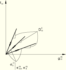
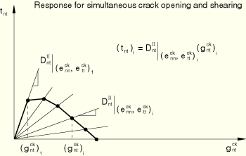
The Mode II model is based on the common observation that the shear behavior is dependent on the amount of crack opening. Therefore, ABAQUS offers a shear retention model in which the postcracked shear stiffness is dependent on crack opening. This model defines the total shear stress as a function of the total shear strain (shear direction ![]() is used as an example):
is used as an example):
![]()
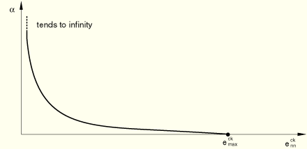
A commonly used mathematical form for this dependence when there is only one crack, associated with direction ![]() , is the power law proposed by Rots and Blaauwendraad (1989):
, is the power law proposed by Rots and Blaauwendraad (1989):
![]()
When the shear component under consideration is associated with only one open crack direction (![]() or
or ![]() ), the crack opening dependence is obtained directly from Figure 4.5.3–8. However, when the shear direction is associated with two open crack directions (
), the crack opening dependence is obtained directly from Figure 4.5.3–8. However, when the shear direction is associated with two open crack directions (![]() and
and ![]() ), then
), then
![]()
![]()
![]()
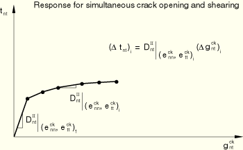
This total stress-strain shear retention model differs from the traditional shear retention models in which the stress-strain relations are written in incremental form (again, shear direction ![]() is used as an example):
is used as an example):