Product: ABAQUS/Standard
Frame elements are designed for the analysis of initially straight, slender beams. The elements are implemented for large displacements and large rotations but small strains. The elastic response of the frame elements follows Euler-Bernoulli beam theory. Plasticity is included in the element's response through a lumped plasticity model with kinematic hardening, which permits yielding only at the ends of the beam. The hardening data are given as a relationship between the generalized force and generalized displacement. Hence, the plastic response of the element is length dependent. The elastic-plastic frame elements are designed to represent plastic hinge formation in frame-like structures, where a single frame element can be used as a member between the structure's nodes.
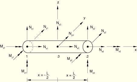
Frame elements are formulated in terms of the solution variables at user-defined end nodes and extra internal degrees of freedom associated with an internal node. The three-dimensional version of the element is discussed here. The two-dimensional version is found by appropriate reduction of the three-dimensional degrees of freedom. The element has three nodes (two user-defined and one internal), 12 external degrees of freedom, and three internal degrees of freedom. Each of the two end nodes has six external degrees of freedom: three displacements and three rotations. An internal node (at the center of the element) has three displacement degrees of freedom only, as shown in Figure 3.9.2–1.
The element is formulated in a local system with the ![]() -direction representing the axial direction and the
-direction representing the axial direction and the ![]() - and
- and ![]() -directions representing the directions transverse to the frame element axis. In this local coordinate system the element's degrees of freedom can be written
-directions representing the directions transverse to the frame element axis. In this local coordinate system the element's degrees of freedom can be written
![]()
![]()
The elastic response of the element is governed by Euler-Bernoulli beam theory. The displacement interpolation for the deflections transverse to the frame element axis (the ![]() - and
- and ![]() -directions) uses fourth-order polynomials, allowing for quadratic variation of the curvature along the beam axis. Let
-directions) uses fourth-order polynomials, allowing for quadratic variation of the curvature along the beam axis. Let ![]() be the isoparametric coordinate along the length of the beam. Then,
be the isoparametric coordinate along the length of the beam. Then,
![]()
![]()
The transverse displacement interpolations incorporate exact solutions to force and moment loading at the ends and constant distributed loads along the beam axis (such as gravity loading). The displacement interpolation function along the frame element axis (the ![]() -direction) is a second-order polynomial, allowing for linear variation of the axial strain along the frame element axis:
-direction) is a second-order polynomial, allowing for linear variation of the axial strain along the frame element axis:
![]()
The twist rotation degree of freedom interpolation along the beam axis (rotation about the ![]() -axis) is linear, allowing for constant twist strain:
-axis) is linear, allowing for constant twist strain:
![]()
The generalized strains, following Euler-Bernoulli beam theory, are
![]()
![]()
The strain-displacement relationship is written in matrix form as
![]()
![]()
The elastic stiffness matrix is integrated numerically and used to calculate 15 nodal forces and moments—12 forces/moments (also called generalized forces) associated with the two end nodes,
![]()
![]()
![]()
![]()
The elastic stiffness is, therefore, a ![]() matrix relating the force vector,
matrix relating the force vector, ![]() , and the nodal displacement vector,
, and the nodal displacement vector, ![]() :
:
![]()
Material properties of frame elements can, in general, be temperature dependent. Let us define the elastic strain vector as
![]()
![]()
![]()
is the thermal expansion coefficient,
![]()
is the current temperature at the frame element section,
![]()
is the reference temperature for ![]() , and
, and
![]()
is the user-defined initial temperature at this point (“Initial conditions,” Section 19.2.1 of the ABAQUS Analysis User's Manual).
Initial generalized strains, ![]() , are calculated from the initial generalized forces given by the user, using the relationship
, are calculated from the initial generalized forces given by the user, using the relationship
![]()
![]()
ABAQUS integrates the elastic stiffness matrix numerically:
![]()
For the simplest case of a temperature-independent material and a pipe cross-section, the elastic stiffness matrix can be integrated analytically to give:
Twisting moments at the end nodes:
![]()
Axial forces at the nodes:
Bending moments at the end nodes and transverse forces for all three nodes:
We assume that the displacement and rotation increments admit an additive decomposition into elastic and plastic parts. Hence,
![]()
![]()
Introduce the lumped plasticity concept such that plastic deformation can develop at the beam external (end) nodes only and develops through plastic rotations (hinges) and plastic axial displacement at one or both nodes. Further assume that the plastic deformation at the external nodes can be caused by the interaction of all three moments and the axial force. Therefore, the vector of plastic deformation at those end nodes has the following form:
![]()
![]()
![]()
![]()
![]()
![]()
![]()
![]()
The hardening model follows a nonlinear kinematic hardening rule generalized from the linear Ziegler hardening law and the relaxation term (the recall term), which introduces the nonlinearity. For details on the hardening model, see “Models for metals subjected to cyclic loading,” Section 4.3.5. Now introduce the generalized backstress vector, ![]() , which defines the origin of the moving plastic interaction surface, and define it as
, which defines the origin of the moving plastic interaction surface, and define it as
![]()
![]()
![]()
![]()
Plastic interaction surfaces formulated in the generalized sectional variables depend on the cross-section profile. Frame elements with lumped plasticity are valid for tubular cross-sections only, and in the simplest form the interaction surface can be expressed as an ellipsoid in a space of four sectional components: axial force and three moments. Normalized with the ultimate forces and moments for each of the sectional components, the plastic interaction surface, ![]() , can be written for each end
, can be written for each end ![]() of the frame element as
of the frame element as
![]() and
and ![]() , the frame element stays elastic.
, the frame element stays elastic.
![]() and
and ![]() , the frame element is elastic-plastic. If the plastic condition at the end
, the frame element is elastic-plastic. If the plastic condition at the end ![]() is exceeded, an iterative procedure is needed to find the final deformation state at the end of the increment. Either end
is exceeded, an iterative procedure is needed to find the final deformation state at the end of the increment. Either end ![]() stays elastic and end
stays elastic and end ![]() becomes plastic, or both ends become plastic.
becomes plastic, or both ends become plastic.
![]() and
and ![]() , the frame element is elastic-plastic. If the plastic condition is exceeded at one or both nodes, an iterative procedure is needed to find the final deformation state at the end of the increment. Depending upon the ratio of plastic deformation at both ends, one or both ends will become plastic.
, the frame element is elastic-plastic. If the plastic condition is exceeded at one or both nodes, an iterative procedure is needed to find the final deformation state at the end of the increment. Depending upon the ratio of plastic deformation at both ends, one or both ends will become plastic.
The integration of the plasticity model for frame elements follows the same general rule as described in “Integration of plasticity models,” Section 4.2.2.
To solve for the value of the deformation and sectional forces at the end of the increment for an arbitrary load increment, an iterative process is required. To set up an appropriate Newton loop, the following relationships are used, with some of them linearized:
Elastic equilibrium equation:
The associated flow rule:
The hardening evolution law:
The backstress definition:
The plastic interaction surfaces at both frame ends:
The frame elements admit large overall displacements and rotations; however, it is assumed that the strains are small. Accordingly, the nonlinear geometric formulation corresponds to Euler-Bernoulli beam theory superposed on a rotating reference frame. An Euler-Bernoulli displacement field, ![]() , is defined relative to this rotation reference configuration, which causes straining. The Euler-Bernoulli displacement field is defined as follows.
, is defined relative to this rotation reference configuration, which causes straining. The Euler-Bernoulli displacement field is defined as follows.
Let ![]() and
and ![]() be the average position and average rotation of the frame element in the deformed configuration:
be the average position and average rotation of the frame element in the deformed configuration:
![]()
![]()
![]()
![]()
To define the strain-inducing rotation contributions, we multiplicatively decompose the rotation at each node,
where![]()
![]()
![]()
The Euler-Bernoulli displacement field is the difference between the position of the node relative to the element center and the reference position of the node relative to the reference center rotated to the current configuration by the average rotation:
![]()
![]()
![]()
![]()
![]()
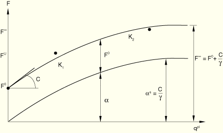
The user can supply hardening data for sectional forces in the form of pairs of values relating the axial nodal force to the plastic extension and the bending and twisting moments to the plastic rotations. If both the hardening data and the yield stress value for the frame section are omitted, ABAQUS assumes that the frame element will remain elastic.
The curve fitting algorithm is used for the evolution hardening equation. At least three pairs of data are required for ABAQUS to fit the curve and solve for the constants ![]() and
and ![]() for each generalized force component,
for each generalized force component, ![]() , as shown in Figure 3.9.2–2.
, as shown in Figure 3.9.2–2.
The parameters ![]() are scaled according to the following formula:
are scaled according to the following formula:
![]()