3.6.3 Shear flexible small-strain shell elements

Product: ABAQUS/Standard

This section discusses the formulation of the small-strain shear flexible elements in ABAQUS/Standard, which are quadrilaterals (S4R5, S8R5, S9R5, and S8R), except for the 6-node triangle STRI65. The essential idea of these elements is that the position of a point in the shell reference surface——and the components of a vector —which is approximately normal to the reference surface—are interpolated independently. The kinematics of the shell theory then consist of measuring membrane strain on the reference surface from the derivatives of with respect to position on the surface and bending strain from the derivatives of ; the strain measures that are used for this purpose are approximations to Koiter-Sanders theory strains (Budiansky and Sanders, 1963). The transverse shear strains are measured as the changes in the projections of onto tangents to the shell's reference surface. For these element types the strain measures are suitable for large rotations but small strains, and the change in the shell's thickness caused by deformation is neglected.

Notation

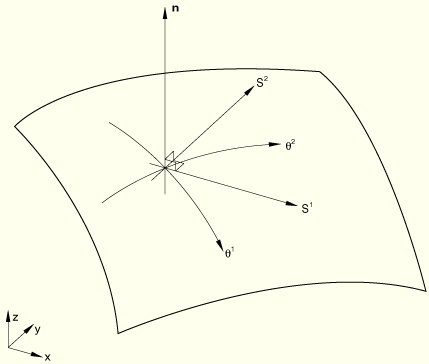
A typical piece of shell surface is shown in Figure 3.6.3–1.

Figure 3.6.3–1 Shell reference surface.

Let (

) be a set of Gaussian surface coordinates on the shell reference surface. Since these coordinates are only needed locally at an integration point, we use the element's isoparametric coordinates as these coordinates.

is the current position of a point on the interpolated reference surface, and

is the initial position of the same point. The unit vector

is the unit normal to the interpolated reference surface in the initial configuration. This vector gives a “sidedness” to the surface—one surface of the shell is the “top” surface (in the positive direction along

from the shell's reference surface) and the other is the bottom surface. The vector corresponding to

in the current configuration,

, will be made approximately normal to the reference surface in the current configuration by imposing the Kirchhoff constraint discretely.

In the rest of this section Greek indices will be used to indicate values associated with the (two-dimensional) reference surface and so will sum over the range 1, 2 under the summation convention.

First, we establish convenient directions for stress and strain output. These will be local material directions, indistinguishable (to the order of approximation) from corotational directions, since we assume strains are small. The standard convention used throughout ABAQUS for such local directions on a surface is as follows.

It is most convenient to choose orthogonal directions. Define

so long as

, where

is a unit vector in the global

-direction; otherwise,

where

is a unit vector in the global

-direction. Then define

Let

so that the

are locally defined distance measuring coordinates at each material point. The transformation

transforms locally with respect to surface coordinates. Here

Stress and strain components are formed in the (, ) directions.

Surface measures

The following surface measures are defined. The metric of the deformed surface is

and an approximation to the curvature tensor (the second fundamental form) is

(this is only an approximation because

is not exactly normal to the surface in the current configuration).

The corresponding measures associated with the original reference surface are the metric

and the approximation to the curvature

The vectors

are defined from the derivatives of the interpolation functions and the “normals” at the nodes. These nodal normals are calculated as average values of the normals to the surfaces of all elements abutting the node. ABAQUS determines if the surface is intended to be smooth at the node (the criterion is that the angle between the normals at the node should be less than 20°). If the surface is not calculated as smooth, separate normals are set up in the different surface branches at the node. Thus,

should be a reasonable approximation to the second fundamental form of the original reference surface.

Displacements

The nodal variables for shell elements are the displacements of the shell's reference surface, , and the normal direction, . Since is defined to be a unit vector, only two independent values are needed to define , so that this type of shell element needs only five degrees of freedom per node. In ABAQUS this issue is addressed in two ways. At nodes in a smooth shell surface in those elements that naturally have five degrees of freedom per node, ABAQUS stores the values of the projections of the change in projected onto two orthogonal directions in the shell surface at the start of the increment to define . Otherwise, ABAQUS stores the usual rotation triplet, , at the node. This latter method leaves a redundant degree of freedom if the node is on a smooth surface. A small stiffness is introduced locally at the node to constrain this extra degree of freedom to a measure of the same rotation of the shell's reference surface.

Interpolation

The same bipolynomial interpolation functions are used for all components of , , , and . The shear flexible shell elements in the library use bilinear interpolation (four nodes), fully biquadratic interpolation (nine nodes), and “serendipity” quadratics (eight nodes).

Strains

The reference surface membrane strains are

The curvature change is

The transverse shears are

where

is a unit vector, tangent to the

line in the current surface.

In addition to these strains, when six degrees of freedom are used at the nodes of the elements, the extra rotation degree of freedom is constrained with a penalty, as follows.

When such a node is the corner node of an element, define , , , , and in the element as above. Notice that these will be different in each element at the node, since the interpolated surface is not generally continuous. Then the strain to be penalized is defined as

where

is the rotated tangent direction, as defined by the rotation values at the node, and

is the rotated tangent direction defined by the motion of the interpolated reference surface at the node.

At each midside node in the original configuration, define as the average surface normal for the elements of this surface branch at the nodes (there will be at most two such elements) and as the tangent to the edge. Then define

as rotated values of

and

, as defined by the rotation values at the node. The vector

is then normal to

and to the edge.

The strain to be penalized at these midside nodes is then defined as

where

is the tangent to the edge of the element in the current position of the reference surface.

Penalties

The transverse shear strains are calculated at a set of reduced integration points and have the following stiffness associated with them:

where the

are the elastic moduli associated with transverse shear. The

are defined directly by the user or are computed from the elastic moduli given for the layers of the shell.

is the shell thickness;

is the value of reference surface area associated with this integration point in the numerical integration scheme;

is a numerical factor, currently set to

. (See Hughes et al., 1977, for a discussion of such factors.) Transverse shears are always treated elastically: nonlinear material calculations in shells are based on plane stress theory, using the membrane and bending strains to define the strain on the surface parallel to the shell's reference surface at each integration point through the shell's thickness.

When rotation constraints are required at nodes that use six degrees of freedom, the penalty used is

This is the same as the transverse shear constraint, except that is here an area “assigned” to the node and the factor is introduced. This (small) factor has been chosen based on numerical experiments, to be large enough to avoid singularities yet small enough to avoid adding significantly to the stiffness of the model.

These strain measures, with the interpolation specified above, give zero strain for any general rigid body motion

where

, and

are constant.

First variations of strain

The first variations of the strains are

where

and at the midside nodes

Second variations of strains

In forming the initial stress matrix we approximate by neglecting , , etc, to simplify the expressions and reduce the cost of forming the matrix. Numerical experiments have suggested that, at least for the problems tested, this does not significantly affect the convergence rate. With this approximation,

and

Internal virtual work rate

For these shell elements the internal virtual work rate is assumed to be

where

, and

are the transverse shear stiffness and the penalties defined above and

indicates the integration points at which transverse shears are calculated,

indicates corner nodes at which six degrees of freedom are used, and

indicates midside nodes at which six degrees of freedom are used. Here

and

are the strain and stress in the (

) material directions in a surface offset by a distance

from the reference surface. The usual Kirchhoff assumption is adopted:

so that the first term above is

The thickness direction integrations are performed numerically in ABAQUS. The integration scheme is a Simpson's rule, of user-chosen order. The shell can also be considered layered, with different properties at each layer and a different integration scheme assigned (by the user) to each layer.

Pressure load stiffness

The load stiffness associated with pressure loading is often important in shells, especially in eigenvalue buckling estimates on elastic shells. In ABAQUS/Standard the pressure load stiffness is implemented as a symmetric form, thus assuming that the pressure magnitude is constant over the surface and neglecting free edge effects. See Hibbitt (1979) and Mang (1980) for details.

The load stiffness is obtained in such a form as follows. The external virtual work associated with pressure is