ABAQUS includes two libraries of axisymmetric membrane elements, MAX and MGAX, whose geometry is axisymmetric (bodies of revolution) and that can be subjected to axially symmetric loading conditions. In addition, MGAX elements support torsion loading and general material anisotropy. Therefore, MGAX elements will be referred to as generalized axisymmetric membrane elements, and MAX elements will be referred to as regular axisymmetric membrane elements. In both cases the body of revolution is generated by revolving a line that represents the membrane surface (a membrane has negligible thickness) about an axis (the symmetry axis) and is described readily in cylindrical coordinates , , and . The radial and axial coordinates of a point on this cross-section are denoted by and , respectively. At , the radial and axial coordinates coincide with the global Cartesian - and -coordinates.

If the loading consists of radial and axial components that are independent of and the material is either isotropic or orthotropic, with being a principal material direction, the displacement at any point will have only radial () and axial () components. The only nonzero stress components are and , where denotes a length measuring coordinate along the line representing the membrane surface on any – plane. The deformation of any – plane (or, more precisely, any – line) completely defines the state of stress and strain in the body. Consequently, the geometric model is described by discretizing the reference cross-section at .

If one allows for a circumferential component of loading (which is independent of ) and general material anisotropy, displacements and stress fields become three-dimensional. However, the problem remains axisymmetric in the sense that the solution does not vary as a function of , and the deformation of the reference – cross-section characterizes the deformation in the entire body. The motion at any point will have—in addition to the aforementioned radial and axial displacements—a twist (in radians) about the -axis, which is independent of . There will also be a nonzero in-plane shear stress, , as a result of the deformation.

This section describes the formulation of the generalized axisymmetric membrane elements. The formulation of the regular axisymmetric membrane elements is a subset of this formulation.

Kinematic description

The coordinate system used with both families of elements is the cylindrical system (, , ), where measures the distance of a point from the axis of the cylindrical system, measures its position along this axis, and measures the angle between the plane containing the point and the axis of the coordinate system and some fixed reference plane that contains the coordinate system axis. The order in which the coordinates and displacements are taken in these elements is based on the convention that is the second coordinate. This order is not the same as that used in three-dimensional elements in ABAQUS, in which is the third coordinate; nor is it the order (, , ) that is usually taken in cylindrical systems.

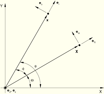
Let , , and be unit vectors in the radial, axial, and circumferential directions at a point in the undeformed state, as shown in Figure 3.2.8–1.

Figure 3.4.3–1 Cylindrical coordinate system and definition of position vectors.

The reference position of the point can be represented in terms of the original radius, , and the axial position, :

Likewise, let , , and be unit vectors in the radial, axial, and circumferential directions at a point in the deformed state. As shown in Figure 3.2.8–1, the radial and circumferential base vectors depend on the coordinate: and .

The current position, , of the point can be represented in terms of the current radius, , and the current axial position, , as

The general axisymmetric motion at a point on the membrane surface can be described by

As this description implies, the degrees of freedom , , and are independent of . Moreover, the reference cross-section of interest is at ; however, for the benefit of the mathematical analysis to follow, it is important that be considered an independent variable in the above expression for .

Parametric interpolation and integration

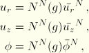
The following isoparametric interpolation scheme is used for the motion:

where is the isoparametric coordinate in the reference – cross-section at ; and , , are the nodal degrees of freedom. The interpolation functions are identical to those used for truss elements (see “Truss elements,” Section 3.4.2). All elements use reduced integration.

Deformation gradient

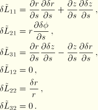
For a material point the deformation gradient is defined as the gradient of the current position, , with respect to the original position, , and is given by

The components of the deformation gradient require that two sets of orthonormal basis vectors be defined. In the undeformed configuration the basis vectors are defined by

where the denote length measuring coordinates in the reference configuration along the element length and the hoop direction, respectively. Thus,

In the current configuration ABAQUS formulates the equations in terms of a fixed spatial basis with respect to the axisymmetric twist degree of freedom. The basis vectors convect with the material. However, because of the axisymmetry of the model in the deformed configuration, these vectors can be defined at as

where the denote length measuring coordinates in the current configuration along the element length and the hoop direction, respectively. Thus, the basis vectors in the reference and current configurations can be written as

where and are length measuring coordinates along the element length in the reference and current configurations, respectively. The components of the deformation gradient in the two sets of basis vectors may be computed as

Using the definitions of the basis vectors in Equation 3.4.3–3, the components of the deformation gradient tensor are

Virtual work

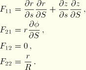
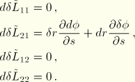
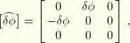
As discussed in “Equilibrium and virtual work,” Section 1.5.1, the formulation of equilibrium (virtual work) requires the virtual velocity gradient, which takes the form

where represents the first variation of the deformation gradient tensor. Alternatively, the virtual velocity gradient can be written as

Recall that ABAQUS formulates the finite element equations in terms of a fixed spatial basis with respect to the axisymmetric twist degree of freedom. Therefore, the desired result for does not simply follow from the linearization of Equation 3.4.3–2. Namely, the contributions from the variations

arising from the spin of the coordinate system must be canceled out. To this end, can be modified according to

where instantaneously, but its variation is given by

where is skew-symmetric with components

with respect to the basis , , and at .

With this modification, the corotational virtual deformation gradient is given by

and the corotational virtual velocity gradient by

The individual components of are given by

The components are not determined by the kinematics.

Stiffness in the current state

The second variation has the usual contribution:

Moreover, there are additional contributions from , which are given by

The remaining terms do not contribute since .