Products: ABAQUS/Standard ABAQUS/Explicit
Submodeling is the technique of studying a local part of a model with a refined mesh, based on interpolation of the solution from an initial, global model onto the nodes on the appropriate parts of the boundary of the submodel. The method is most useful when it is necessary to obtain an accurate, detailed solution in the local region and the detailed modeling of that local region has negligible effect on the overall solution. The response at the boundary of the local region is defined by the solution for the global model and it, together with any loads applied to the local region, determines the solution in the submodel. The technique relies on the global model defining this submodel boundary response with sufficient accuracy.
Submodeling can be applied quite generally in ABAQUS. With a few restrictions different element types can be used in the submodel compared to those used to model the corresponding region in the global model. Both the global model and the submodel can use solid elements, or they can both use shell elements. A special option is available to use a submodel consisting of solid elements with a global model consisting of shell elements. The material response defined for the submodel may also be different from that defined for the global model. Both the global model and the submodel can have nonlinear response and can be analyzed for any sequence of analysis procedures. The procedures do not have to be the same for both models.
The submodel is run as a separate analysis. The only link between the submodel and the global model is the transfer of the time-dependent values of variables to the relevant boundary nodes (the “driven nodes”) of the submodel. The only information in the global model available to the submodel analysis is the file output data written during the global model analysis. It contains, by default, the undeformed coordinates of all global model nodes and element information for all elements in the global model (see “Results file output format,” Section 5.1.2 of the ABAQUS Analysis User's Manual). The user must have requested nodal responses in the area where the submodel boundary is located. These responses are used to prescribe boundary conditions at the driven nodes in the submodel.
In the solid-to-solid case the positions of the submodel boundary nodes (the driven nodes) are determined with respect to the global model, and the appropriate element interpolation functions are used to obtain the values of the degrees of freedom at the driven nodes. An “exterior tolerance,” which the user can specify, is used to check whether it is valid to extrapolate values from the global model. The extrapolation is valid if the distance between the driven nodes and the free surface of the global model falls within the specified tolerance.
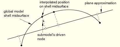
A similar check is done along the global model boundaries for the shell-to-shell submodeling case. We also check whether the driven nodes of the submodel lie sufficiently close to the midsurface of the shell elements in the global model. To simplify the calculations, the closest point in the global model is approximated by measuring the distance in the direction normal to a flat approximation to each shell element in the global model, as shown in Figure 2.15.1–1.
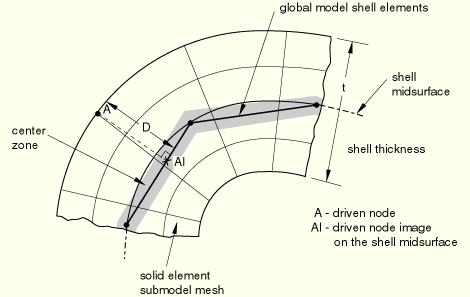
For the shell-to-solid case ABAQUS uses two kinds of tolerances to determine the relation between the submodel and the global model. First, the closest point on the shell midsurface of the global model is determined. This point will subsequently be referred to as the “image node” of the driven node. The exterior tolerance parameter is used to check if the image node lies within the domain of the global model. Then the distance between the driven node and its image is checked against half of the maximum shell thickness specified by the user (see Figure 2.15.1–2).If the node is within the half thickness plus the exterior tolerance, it is accepted. This check is only approximate if the global model has varying shell thickness, and in that case it will not protect the user in parts of the global model that have a small thickness compared to the maximum thickness specified by the user.
After the locations of the driven nodes (or image nodes for the shell-to-solid case) are determined, the prescribed values of the driven variables are interpolated from the values written to the file output for the global model. These must have been written with a sufficiently high frequency to obtain accurate values at the driven nodes. All components of displacements, temperatures, charges, and—for complex steady-state dynamic analysis—the phase angles as well as the amplitudes have to be written for the global model nodes from which the values for the driven nodes will be interpolated. For small global models responses will typically be written for all nodes. For large global models node sets can be created that contain the nodes in the regions around the submodel boundary.
For solid-to-solid and shell-to-shell submodeling, the interpolated values of displacements, rotations, temperatures, etc. are applied directly to the driven nodes. For these nodes the user can specify the individual degrees of freedom that are driven.
In the shell-to-solid case the driven degrees of freedom are chosen automatically, depending on the distance between the driven node and the midsurface of the shell. If the node lies within the center zone (specified by the user; see Figure 2.15.1–2), all displacement components are driven. If the node lies outside the center zone, only the displacement components parallel to the shell midsurface are driven. By default, the size of the center zone is taken as 10% of the maximum shell thickness. The procedure is described in detail below. The center zone should be large enough so that it contains at least one layer of nodes. If the transverse shear stresses at the submodel boundary are high and the submodel is highly refined in the thickness direction, this can result in high local stresses, since the shear force at the submodel boundary is only transferred at the driven nodes within the center zone. High transverse shear stresses occur only in regions where bending moments vary rapidly, and it is better not to locate the submodel boundary in such regions. It is best to locate the submodel boundary in areas of low transverse shear stress in the global model.
All displacement degrees of freedom are driven when the driven node lies within the center zone. For geometrically linear analysis these prescribed displacements are obtained from the displacements and rotations of the image node as
where![]()
For large-displacement analysis finite rotations must be taken into account. The finite rotation equivalent of Equation 2.15.1–1 is
where![]()
For driven nodes outside the center zone only the displacement components parallel to the shell midsurface are driven. For the geometrically linear case this leads to the constraints
whereSince the submodeling capability in ABAQUS is quite general and allows the use of different procedure types in both analyses, there are several possibilities for the evaluation of the values at driven nodes as follows. In all cases ABAQUS assumes that the global model and the submodel both use small- or large-displacement theory.
In the schemes listed below the first procedure type applies to the global analysis and the second to the submodel analysis.
General procedure to general procedure for small-displacement theory: Equation 2.15.1–1 is used inside the center zone, and Equation 2.15.1–3 is used outside the center zone.
General procedure to general procedure for large-displacement theory: Equation 2.15.1–2 is used inside the center zone, and Equation 2.15.1–4 outside the center zone.
General procedure to linear perturbation procedure for small-displacement theory:
inside the center zone, and outside the center zone;General procedure to linear perturbation procedure for large-displacement theory:
inside the center zone, and outside the center zone, whereLinear perturbation procedure to general procedure for small-displacement theory:
inside the center zone, and outside the center zone;Linear perturbation procedure to general procedure for large-displacement theory:
inside the center zone, and outside the center zone. Since the base state is not available, an approximate form is used, whereLinear perturbation procedure to linear perturbation procedure for small-displacement theory:
inside the center zone, and outside the center zone.Linear perturbation procedure to linear perturbation procedure for large-displacement theory:
inside the center zone, and outside the center zone. Since the base state is not available,