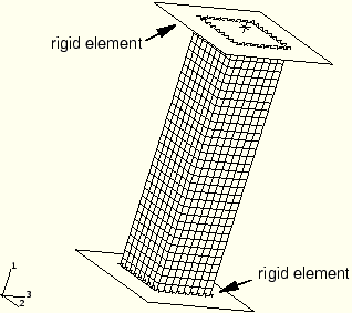
You have been asked to analyze the crushing of a square, steel box tube between two rigid plates, as shown in Figure 6–25. The tube is free at one end, and it is attached to a rigid plate with a 500 kg mass at its other end. Both the tube and the rigid plate with mass have an initial velocity of 8.9408 m/s (20 mph) just before the tube's free end impacts a stationary rigid surface. During impact, the tube dissipates a large amount of the initial kinetic energy into plastic deformation, and your primary interest is in evaluating the tube's ability to absorb kinetic energy. It is important to model the self-contact in the tube correctly as it folds upon itself while buckling. An application for such an analysis would be the design of energy absorption zones in an automobile frame.
Figure 6–26 shows the suggested mesh for this simulation.
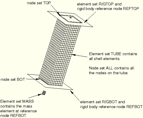
Shell elements are appropriate because the thickness (0.001 m) is 1/100th of the smallest planar dimension (0.1 m). While the initial model contains two symmetry planes, it is important to model the entire structure because it is not known whether the lowest buckling modes are symmetric or unsymmetric. Because the tube's deformation will involve buckling, it is necessary to seed the mesh with the lowest buckling modes of the tube to obtain a smooth postbuckling response. You will obtain the first 10 buckling modes by running an eigenvalue buckling analysis of the tube using ABAQUS/Standard and storing these modes in the results (.fil) file. You will then use the *IMPERFECTION option in ABAQUS/Explicit to read the buckling modes, scale them, and use them to perturb the nodal coordinates.All of the necessary node and element sets are shown in Figure 6–27.
Place the shell elements in an element set called TUBE. Place the top and bottom rigid elements into their own element sets: RIGTOP and RIGBOT. The mass element belongs in an element set called MASS. Place the nodes on the top end of the tube (largest 1-coordinate) in a node set called TOP, and place the nodes on the bottom end of the tube (smallest 1-coordinate) in a node set called BOT. You will use these node sets later when defining interactions with the rigid plates. Create a node set called ALL containing all of the nodes on the tube. You will use this node set when defining the initial velocity of the tube.Use your preprocessor to generate the mesh shown in Figure 6–26, which is 8 elements wide and 32 elements long. Use S4R elements to model the tube and R3D4 elements to model the rigid plates. Each of the shell elements is 0.0125 m × 0.0125 m, and the rigid elements are 0.2 m × 0.2 m. Define the shell elements such that the normals all point outward. Define a mass element with a mass of 500 kg at the rigid body reference node of the bottom rigid body. In the ABAQUS/Explicit analysis you will give the mass element and the tube an initial velocity, and its momentum will cause the tube to crush against the top rigid plate. This mass element is not necessary for the ABAQUS/Standard analysis, which is static; however, it does no harm to include the mass in both input files.
Before creating the input file for the ABAQUS/Explicit analysis, you must create the input file for the ABAQUS/Standard buckling analysis. The buckling analysis should contain as nearly as possible the same mesh and boundary conditions as the crushing analysis. The following would be a suitable description in the *HEADING option for the buckling analysis in ABAQUS/Standard:
*HEADING
Tube crush (x-direction) -- buckling analysis
Tube dimensions: 0.4m x 0.1m x 0.1m
SI units (kg, m, s, N)
Section properties
All of the shell elements in the model have the same material and the same 0.001 m (1 mm) thickness. For efficiency use the default Simpson's integration rule with the minimum of three integration points through the shell thickness. While more integration points increases the accuracy of the solution, it also increases its expense. Use the following section property for the shell elements:
*SHELL SECTION, ELSET=TUBE, MATERIAL=STEEL
0.001, 3
The rigid elements also require section properties. Use the following section properties for the two rigid bodies:
*RIGID BODY, ELSET=RIGTOP, REF NODE=<top reference node number>
*RIGID BODY, ELSET=RIGBOT, REF NODE=<bottom reference node number>
The mass element also requires section properties. Use the following section property to define a 500 kg mass attached to the bottom rigid body reference node:
*MASS, ELSET=MASS
500.,
Material properties
The tube is made of steel, which will be modeled as an isotropic, elastic-plastic material. Plasticity data and density are not necessary for the buckling analysis, which uses only the linear material properties. However, include the data anyway for consistency with the ABAQUS/Explicit input file. ABAQUS/Standard ignores any material options that are not relevant. Use the following material option block to define the material behavior:
*MATERIAL, NAME=STEEL
*ELASTIC
207.E9, .3
*PLASTIC
1.587E8, 0.0
1.631E8, 0.015
1.863E8, 0.033
1.932E8, 0.044
2.020E8, 0.062
2.070E8, 1.500
*DENSITY
7800.,
Initial conditions
There are no initial conditions because you do not need to include the initial velocity in the buckling analysis.
Boundary conditions
Constrain the top rigid body completely by constraining its reference node.
*BOUNDARY
REFTOP, 1, 6
Constrain the bottom rigid body in all but the 1-degree of freedom by constraining its reference node.
REFBOT, 2, 6
Contact definitions
Define surfaces on the top and bottom rigid elements. The surfaces must be on the side of the elements facing the tube, which may be either the SPOS or the SNEG face, depending on how you defined the rigid elements.
*SURFACE, NAME=TOPSU
RIGTOP, <SPOS or SNEG>
*SURFACE, NAME=BOTSU
RIGBOT, <SPOS or SNEG>
Create a node-based surface using the nodes at the top of the tube (contained in node set TOP).
*SURFACE, TYPE=NODE, NAME=TOP
TOP,
Define contact between the nodes at the top of the tube and the top rigid surface. In a linear perturbation step, such as *BUCKLE, the contact conditions at the start of the step remain unchanged throughout the step. Therefore, if you ensure that the top nodes of the tube are in contact with the top rigid surface at the start of the step, the contact constraint will remain in effect throughout the buckling analysis. To ensure the closed contact condition, use the ADJUST parameter, which moves nodes within the specified tolerance (0.01 m) to lie exactly on the contact surface.
*CONTACT PAIR, ADJUST=0.01, INTERACTION=TUBE
TOP, TOPSU
A contact pair must refer to a *SURFACE INTERACTION option, which may contain additional information regarding the contact interaction, such as a friction model. In this case we assume zero friction between the tube and the top rigid surface. The *SURFACE INTERACTION option block contains only the following keyword line:
*SURFACE INTERACTION, NAME=TUBE
Create a node-based surface containing the nodes at the bottom of the tube.
*SURFACE, TYPE=NODE, NAME=BOT
BOT,
Tie constraints
Use the *TIE option to “glue” the slave nodes on the bottom of the tube to the bottom rigid surface. To ensure that the slave nodes are tied to the bottom rigid surface, set the ADJUST parameter equal to YES and the POSITION TOLERANCE parameter to 0.01. Slave nodes of the tube that are within this tolerance are tied to the bottom rigid surface.
*TIE, NAME=FIXEDBOTTOM, POSITION TOLERANCE=0.01,
ADJUST=YES
BOT, BOTSU
Step definition
To obtain the first 10 buckling modes, use the following step definition:
*STEP
Buckling analysis of the tube
*BUCKLE, EIGENSOLVER=SUBSPACE
10,
The subspace iteration eigensolver is used since the Lanczos eigensolver is not suitable for solving a buckling problem with contact conditions.
Loading
Load the tube in a manner similar to the actual loading that the tube will experience during the crushing analysis. The actual load magnitude is not critical because ABAQUS/Standard will report the buckling loads as a fraction of the applied load. Apply a concentrated force of 500 N in the positive 1-direction to the bottom rigid surface reference node:
*CLOAD
REFBOT, 1, 500.0
Output requests
You must request results (.fil) file output for the nodal displacements so that you can use the buckling analysis results to seed the ABAQUS/Explicit mesh with imperfections. In addition, request preselected field variable output to the output database (.odb) file and prevent unnecessary results from being printed in the data (.dat) file.
*NODE FILE
U,
*OUTPUT, FIELD, VARIABLE=PRESELECT, FREQUENCY=1
*NODE PRINT, FREQUENCY=0
*EL PRINT, FREQUENCY=0
*END STEP
After storing your input in a file called tube_buckle.inp, run the analysis using the following command:
abaqus job=tube_buckleIf your analysis does not complete, check tube_buckle.dat for error messages. Modify your input to remove any errors.
After running the buckling analysis to completion, look at the eigenvalue output in the data file. The output shows 10 eigenmodes and 10 corresponding eigenvalues. To determine the actual buckling load, multiply the eigenvalue by the applied load; e.g., the buckling load for the first mode is 35.377 × 500.0 N=17689 N.
                              E I G E N V A L U E    O U T P U T

 BUCKLING LOAD ESTIMATE = ("DEAD" LOADS) + EIGENVALUE * ("LIVE" LOADS).
          "DEAD" LOADS = TOTAL LOAD BEFORE  *BUCKLE STEP.
          "LIVE" LOADS = INCREMENTAL LOAD IN *BUCKLE STEP

 MODE NO      EIGENVALUE

       1       35.377
       2       47.316
       3       47.316
       4       60.433
       5       64.596
       6       66.441
       7       76.665
       8       78.725
       9       87.067
      10       87.069
Postprocessing with ABAQUS/Viewer
Start ABAQUS/Viewer by entering the command
abaqus viewer odb=tube_buckleat the operating system prompt.
View the deformed shape of the eigenmodes, and determine whether the deformations in the buckling analysis will provide good imperfection seeds for the crushing analysis in ABAQUS/Explicit.
To plot the eigenmodes:
From the main menu bar, select Tools![]() Display Group
Display Group![]() Create.
Create.
In the dialog box that appears, select element set PART-1-1.TUBE and click Replace.
Click Dismiss.
Observe that the tube alone is now displayed.
From the main menu bar, select Result![]() Step/Frame.
Step/Frame.
To select the first eigenmode, choose Mode 1 in the dialog box that appears, and click OK.
Change the plot mode to deformed by selecting Plot![]() Deformed Shape or by clicking the
Deformed Shape or by clicking the ![]() tool in the toolbox.
tool in the toolbox.
The first eigenmode is displayed in the viewport.
To change the view, click the rotate tool ![]() and drag the cursor to rotate the tube in the viewport.
and drag the cursor to rotate the tube in the viewport.
Click Deformed Shape Plot Options in the prompt area.
The Deformed Shape Plot Options dialog box appears.
In this dialog box, choose the Hidden render style. Click OK.
The eigenmode is displayed with the changed deformed plot options.
Repeat Step 5 for the second eigenmode.
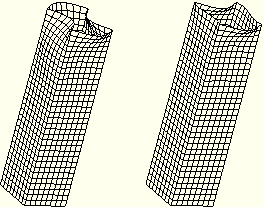
Eigenmodes 1 and 2, which are displayed in Figure 6–28, show that the eigenmodes are similar to the expected deformation during the crushing analysis. Examination of the remaining eight modes shows that they are relevant as well.
Now that you have obtained the buckling modes using ABAQUS/Standard, you are ready to create the ABAQUS/Explicit input file.
Most of the model data are the same for the ABAQUS/Standard buckling analysis and the ABAQUS/Explicit crushing analysis. Specifically, the nodes, elements, material, and section properties are all the same. Also, the tie constraint is the same. One significant difference in the contact definitions is that for ABAQUS/Standard the contact pair definition is part of the model data, whereas in ABAQUS/Explicit the contact pair definition is part of the history data. In addition, the ABAQUS/Explicit input file contains an additional contact pair to model self-contact of the tube as well as an option to read the imperfections from the buckling analysis and to alter the mesh accordingly. The ABAQUS/Explicit model also contains an initial velocity that causes it to impact with the top rigid surface. Copy the buckling input file, tube_buckle.inp, to a file called tube_crush.inp, and then modify tube_crush.inp as described in the next section.
Use the buckling eigenmodes to perturb the mesh
When choosing perturbation magnitudes, the goal is to seed the mesh with a deformation pattern that will allow the postbuckling deformation to proceed correctly. Typically, the magnitudes of the perturbations used for the different eigenmodes are a few percent of the relevant structural dimension, such as shell thickness. Since the lowest eigenmodes are most pertinent to a crushing analysis, the magnitude of the perturbation associated with those modes should be greatest. Increasing the imperfection factors causes the crushing to proceed more smoothly. On the other hand, imperfections that are too large are unrealistic.
The postbuckling response of a structure with many closely spaced eigenvalues may be highly sensitive to the mesh imperfections that you impose. In such cases slight changes to the mesh imperfections can cause significant changes in postbuckling behavior, requiring a sensitivity study to determine realistic mesh imperfections. In this tube crushing analysis the first eigenvalue is significantly lower than the second, so we can safely assume that the first eigenmode will dominate. Only modes 2 and 3 have closely spaced eigenvalues, but these are far enough away from the lowest eigenvalue that they will not dominate the postbuckling response. A structure such as a short, thin-walled cylinder may have several low eigenvalues that are nearly the same. In such a structure it is not clear whether the lowest eigenmode will dominate.
Introduce mesh imperfections that are a maximum of 2% of the shell thickness. Since ABAQUS/Standard scales the eigenvalue output from the buckling analysis so that the maximum deformation in each eigenmode is 1.0 m, choosing an imperfection factor of 1.0 would perturb the mesh by exactly the displacements obtained as output from ABAQUS/Standard. To obtain mesh imperfections for each eigenmode that are a maximum of 2% of the shell thickness (0.001 m × 0.02 = 2.0 × 10⁻⁵ m) for the first eigenmode and a decreasing percentage as the eigenmode number increases, use the following imperfection factors:
*IMPERFECTION, FILE=tube_buckle, STEP=1
1, 2.0E-5
2, 0.8E-5
3, 0.4E-5
4, 0.18E-5
5, 0.16E-5
6, 0.10E-5
7, 0.10E-5
8, 0.08E-5
9, 0.02E-5
10, 0.02E-5
Initial conditions
The top rigid body is fixed. The tube and bottom rigid body, including the mass, have an initial velocity of 20 mph, or 8.9408 m/s. Use the following option block to define the initial velocity:
*INITIAL CONDITIONS, TYPE=VELOCITY
** 1 mph = 0.44701 m/s
** 20 mph = 8.9408 m/s
REFBOT, 1, 8.9408
ALL, 1, 8.9408
Boundary conditions
The boundary conditions are exactly the same as those used for the buckling analysis.
Output node set
Define a node set to use later when requesting output.
*NSET, NSET=PRIN
TOP, REFTOP, BOT, REFBOT
Surface definitions
As the tube crushes, it buckles repeatedly so that many regions on the inside and on the outside of the tube contact each other. Since we do not know in advance which specific regions will be in contact with each other, we must allow contact to occur in a very general manner so that any regions can contact any other regions, both on the inside and on the outside of the tube. We will define the contact conditions in this example using the self-contact and double-sided contact features of the contact pair algorithm in ABAQUS/Explicit. Alternatively, the general contact algorithm could be used.
Delete the surface TOP, the contact pair between surfaces TOP and TOPSU, and the surface interaction TUBE. Define the entire inside and outside surfaces of the tube to be in one double-sided contact surface by defining a shell surface on the element set, TUBE, without specifying a face identifier.
*SURFACE, NAME=TUBE
TUBE,
We now discuss the history data required for this problem, including the step definition, contact definitions, and output requests.
Step definition
Run the explicit dynamics analysis for a total of 0.03 seconds.
*STEP
Impact of square tube with free deceleration
Initial velocity=8.9408m/s (20mph)
*DYNAMIC, EXPLICIT
, 0.03
Contact definitions
To specify self-contact for the inside and outside of the tube, define a contact pair with the double-sided surface, TUBE, as the only surface.
*CONTACT PAIR, INTERACTION=SELF
TUBE,
In addition, define the surface interaction, SELF, with a friction coefficient of 0.1.
*SURFACE INTERACTION, NAME=SELF
*FRICTION
0.1,
Initially, the contact will occur only at the nodes along the top edge of the tube; but as the tube crushes, more of the tube surface could contact the rigid plate. We can define this contact situation by specifying contact between the double-sided surface, TUBE, and the top rigid plate surface, TOPSU. Since a double-sided surface automatically includes the edge in the surface definition, the contact pair is defined as follows:
*CONTACT PAIR, INTERACTION=IMPACT
TUBE, TOPSU
In addition, define the surface interaction, IMPACT, with zero friction.
*SURFACE INTERACTION, NAME=IMPACT
Output requests
Since the primary goal of this analysis is to determine the amount of energy absorbed by the tube as it is crushed, the most important output is the energy history output. Request the following history output to the output database:
*OUTPUT, HISTORY, TIME INTERVAL=0.00008
*ENERGY OUTPUT
ALLWK, ALLKE, ETOTAL, ALLPD, ALLIE, ALLVD, ALLAE, ALLSE
Nodal histories and a monitor node, as well as output of the preselected field variables to the output database, are also useful in studying the behavior of the tube.
*NODE OUTPUT, NSET=PRIN
U, V, A, RF1, RF2, RF3
*MONITOR, NODE=<bottom rigid reference node number>, DOF=1
*OUTPUT, FIELD, VARIABLE=PRESELECT, NUMBER INTERVAL=20
*END STEP
After storing your input in a file called tube_crush.inp, run the analysis using the following command:
abaqus job=tube_crush analysisThis analysis will take a while to complete. If your analysis does not complete, check the data file, tube_crush.dat, and the status file, tube_crush.sta, for error messages. Modify your input to remove any errors.
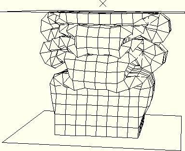
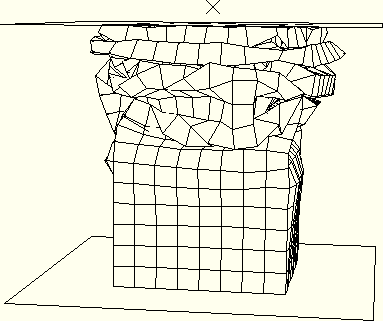
After running the simulation successfully, visually display the deformation history of the tube with an animation using the same procedure that you used to animate the circuit board problem. The animation will show the deformed mesh for each of the 20 states stored in the output database file. Viewing the deformation history enables you to determine whether or not the tube appears to be deforming correctly as it is crushed. The final deformed mesh is shown in Figure 6–29. As you view the displaced mesh, notice that ABAQUS/Explicit includes the thickness of the shell in the contact calculations. The regions that are in contact appear with a slight gap between contacting regions.
To underscore the importance of perturbing the mesh prior to performing a postbuckling analysis, Figure 6–30 shows the final deformed mesh of an analysis that includes no initial imperfections.
In contrast to the smoothly buckled shape of the perturbed mesh, this unperturbed mesh deforms into sharp folds; the shape is clearly not physically correct. Even the small imperfections introduced in the perturbed mesh are enough to make the postbuckling behavior proceed smoothly.Status file
The status file issues several warnings regarding high out-of-plane warping in some surfaces. Such warnings are not surprising considering the severe deformation of the mesh in Figure 6–29. The nature of this crushing analysis is such that a highly refined mesh would be required to eliminate the large warping of some elements. Without further refining the mesh for this exercise, we can simply accept the results as an approximate solution.
  STEP 1  ORIGIN 0.00000E+00

   Total memory used for step 1 is approximately 1.6 megawords
   Global time estimation algorithm will be used.
   Scaling factor :  1.0000

             STEP      TOTAL       CPU     STABLE      CRITICAL  KINETIC
  INCREMENT  TIME      TIME        TIME   INCREMENT    ELEMENT   ENERGY    MONITOR
         0  0.000E+00 0.000E+00   00:00:02 1.392E-06     101   2.003E+04 0.000E+00
 Results number  0 at increment zero.
 ODB Field Frame Number    0 of   20 requested intervals at increment zero.


 ***WARNING: Master surface TUBE of contact pair # 1 contains facets with
             out-of-plane warping of at least 20.000 degrees in increment 320.
             Large warping that develops during an analysis often corresponds
             to severe distortion of the underlying elements. It may be
             appropriate to rerun the analysis with a refined mesh.
Postprocessing with ABAQUS/Viewer
Start ABAQUS/Viewer by entering the command
abaqus viewer odb=tube_crushat the operating system prompt.
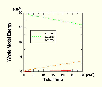
One way to determine the energy absorption of the tube is to look at a history plot of the pertinent energies. Since most of the energy is dissipated in the form of plastic deformation, plot a history of plastic dissipation, ALLPD. To show how the total kinetic energy of the model changes as the tube deforms, also plot kinetic energy, ALLKE. It is also useful to plot the artificial strain energy, ALLAE, as an indication of the mesh quality.
To plot the energy histories:
From the main menu bar, select Result![]() History Output.
History Output.
The History Output dialog box appears.
Select the artificial energy, ALLAE, and save the data as ALLAE.
Select the kinetic energy, ALLKE, and save the data as ALLKE.
Select the plastic dissipation, ALLPD, and save the data as ALLPD.
Click Dismiss to close the dialog box.
From the main menu bar, select Tools![]() XY Data
XY Data![]() Manager.
Manager.
The XY Data Manager dialog box appears.
In this dialog box, select the three curves defined above and click Plot.
Customize the appearance of the plot by changing the curve styles and the axis titles, as shown in Figure 6–31.
By the end of the analysis 3600 J of energy has been dissipated as plastic deformation, and there is a corresponding decrease of 4400 J in the total kinetic energy of the model. The artificial strain energy at the end of the analysis is 800 J, or 18% of the plastic dissipation. Ideally the artificial strain energy should be a much smaller percentage of the internal energy or plastic dissipation. (In previous examples we introduced 5% as a general rule.) The high percentage in this analysis indicates that the mesh should be refined to improve the results. Since the deformations by the end of the analysis are so severe, a highly refined mesh would be required to minimize the effect of hourglassing on the results. Again, without further refining the mesh, we can accept the results as an approximate solution.