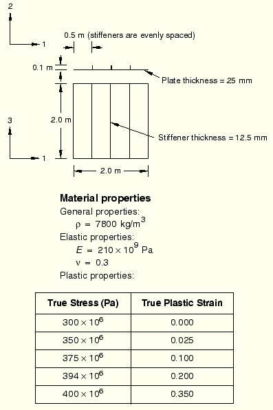
In this example you will assess the response of a stiffened square plate subjected to a blast loading. The plate is firmly clamped on all four sides and has three equally spaced stiffeners welded to it. The plate is constructed of 25 mm thick steel and is 2 m square. The stiffeners are made from 12.5 mm thick plate and have a depth of 100 mm. Figure 5–7 shows the plate geometry and material properties in more detail.
The purpose of this example is to determine the response of the plate and to see how it changes as the sophistication of the material model increases. Initially, we analyze the behavior with the standard elastic-plastic material model. Subsequently, we study the effects of including material damping and rate-dependent material properties.
Use the default rectangular coordinate system with the plate lying in the 1–3 plane. Since the plate thickness is significantly smaller than any other global dimensions, you can use shell elements of type S4R for the model.
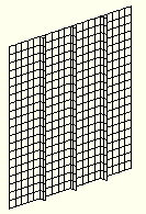
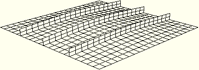
Create your mesh based on the design shown in Figure 5–8, which is a relatively coarse mesh of 20 × 20 elements in the plate and 2 × 20 elements in each of the stiffeners. This mesh corresponds to the input file shown in “Blast loading on a stiffened plate,” Section A.5. It provides moderate accuracy while keeping the solution time to a minimum. Define the mesh so that the element normals for the plate all point in the positive 1-direction. Doing so ensures that the stiffeners lie on the SPOS face of the plate, which will be important when defining the element properties and shell offsets later.
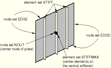
Figure 5–9 shows all the sets necessary to apply the element properties, loads, and boundary conditions.
Include all the nodes on the perimeter of the plate in a node set called EDGE. These nodes will have a completely fixed boundary condition. Define a node set for output purposes called NOUT containing the node at the center of the plate. Put the plate elements in an element set called PLATE, and put the stiffener elements in an element set called STIFF. In addition, define an element set for output purposes called STIFFMAX, which contains the four center elements on the central stiffener. These elements will be subject to the maximum bending stress in the stiffeners.We now review the model data for this problem, including the model description, node and element definitions, element properties and shell offsets, material properties, boundary conditions, and amplitude definition for the blast load.
Model description
The *HEADING option is used to include a title and model description in the input file. The heading is useful for future reference purposes and may contain information on model revisions and the evolution of complex models. It can be several lines long, but only the first line will be printed as a title on the output pages. Below is the *HEADING definition that might be used for this analysis.
*HEADING
Blast load on a flat plate with stiffeners
S4R elements (20x20 mesh)
Normal stiffeners (20x2)
SI units (kg, m, s, N)
Nodal coordinates and element connectivity
Use your preprocessor to generate the mesh shown in Figure 5–8 and the sets shown in Figure 5–9.
Element properties and shell offset
Give each element set the section properties shown below. Include the appropriate MATERIAL parameter on each *SHELL SECTION option so that each set of elements refers to a material definition.
*SHELL SECTION, MATERIAL=STEEL, ELSET=PLATE, OFFSET=SPOS
0.025,
*SHELL SECTION, MATERIAL=STEEL, ELSET=STIFF
0.0125,
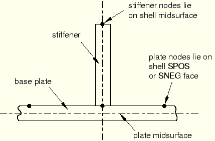
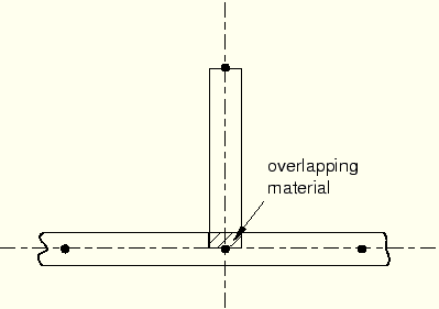
The material named STEEL will be defined in the next section. Setting OFFSET to SPOS offsets the midsurface of the plate one half of the shell thickness away from the nodes. The effect is to make the PLATE nodes lie on the SPOS shell face instead of on the shell midsurface. The purpose of the shell offset in this case is to allow the stiffeners to butt up against the plate without overlapping any material with the plate. Figure 5–10 shows the cross-section of the joint between the stiffener and panel using the OFFSET parameter.
If the stiffener and base plate elements are joined at common nodes at their midsurfaces, an area of material overlaps, as shown in Figure 5–11.
If the thicknesses of the plate and stiffener is small in comparison to the overall dimensions of the structure, this overlapping material and the extra stiffness it would create has little effect on the analysis results. However, if the stiffener is short in comparison to its width or to the thickness of the base plate, the additional stiffness of the overlapping material could affect the response of the whole structure.Material properties
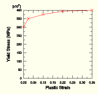
Assume that both the plate and stiffeners are made of steel (Young's modulus of 210.0 GPa and Poisson's ratio of 0.3). At this stage we do not know whether there will be any plastic deformation, but we know the value of the yield stress and details of the post-yield behavior for this steel. We will add this information on the *PLASTIC option in the material definition. The initial yield stress is 300 MPa, and the yield stress increases to 400 MPa at a plastic strain of 35%. The plasticity data are shown below, and the plasticity stress-strain curve is shown in Figure 5–12.
*MATERIAL, NAME=STEEL
*ELASTIC
210.0E9, .3
*PLASTIC
300.0E6, 0.000
350.0E6, 0.025
375.0E6, 0.100
394.0E6, 0.200
400.0E6, 0.350
*DENSITY
7800.0,
During the analysis ABAQUS calculates values of yield stress from the current values of plastic strain. As discussed earlier, the process of lookup and interpolation is most efficient when the data are regular—when the stress-strain data are at equally spaced values of plastic strain. To avoid having the user input regular data, ABAQUS/Explicit automatically regularizes the data. In this case the data are regularized by ABAQUS/Explicit by expanding to 15 equally spaced points with increments of 0.025.
To illustrate the error message that is produced when ABAQUS/Explicit cannot regularize the material data, try setting the regularization tolerance, RTOL, to 0.001 and include one additional data pair, as shown below:
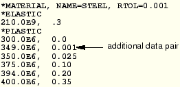
***ERROR: Failed to regularize material data. Try
regularizing the independent variable intervals.
Boundary conditions
Fully constrain the edges of the plate using the node set EDGE defined previously.
*BOUNDARY
EDGE, ENCASTRE
Alternatively, you could specify the degrees of freedom by number.
*BOUNDARY
EDGE, 1, 6
Amplitude definition for blast load
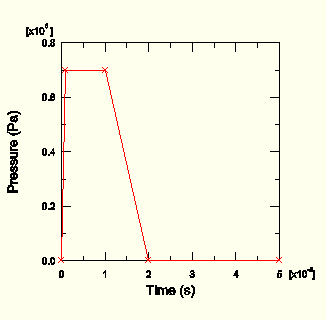
Since the plate will be subjected to a load that varies with time, you must define an appropriate amplitude curve to describe the variation. Define the amplitude curve shown in Figure 5–13 as follows:
*AMPLITUDE, NAME=BLAST 0.0, 0.0, 1.0E-3, 7.0E5, 10E-3, 7.0E5, 20E-3, 0.0 50E-3, 0.0The pressure increases rapidly from zero at the start of the analysis to its maximum of 7.0 × 10⁵ N in 1 ms, at which point it remains constant for 9 ms before dropping back to zero in another 10 ms. It then remains at zero for the remainder of the analysis.
The history data begin with the *STEP option, which is followed immediately by a title for the step. After the title, specify the *DYNAMIC, EXPLICIT procedure with a time period of 50 ms.
*STEP
Apply blast loading
** Explicit analysis with a time duration of 50 ms
*DYNAMIC, EXPLICIT
, 50E-03
Applying the blast load
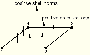
Use the *DLOAD option to apply the blast load to the plate. It is important to ensure that the pressure load is being applied in the correct direction. Positive pressure is defined as acting in the direction of the positive shell normal. For shell elements the positive normal direction is obtained using the right-hand rule about the nodes of the element, as shown in Figure 5–14. Since the magnitude of the load has been defined in the BLAST amplitude definition, you need to apply only a unit pressure under *DLOAD. Apply the pressure so that it pushes against the top of the plate (where the stiffeners are on the bottom of the plate). Such a pressure load will place the outer fibers of the stiffeners in tension. Use the following option in your input file:
*DLOAD, AMPLITUDE=BLAST
PLATE, P, 1.0
Output requests
To check on the progress of the solution, use the *MONITOR option to monitor the deflection at the center node of the plate during the analysis. Monitor the out-of-plane displacement at the center node by adding the following command to your input file:
*MONITOR, NODE=<center node number>, DOF=1Set the number of intervals during the step at which preselected field data are written to the output database file (ODB) to 25. This ensures that the selected data outputs are written every 2 ms since the total time for the step is 50 ms. In general, you should try to limit the number of frames written during the analysis to keep the size of the output database file reasonable. In this analysis saving information every 2 ms should provide sufficient detail to study the response of the structure visually.
*OUTPUT, FIELD, NUMBER INTERVAL=25, VARIABLE=PRESELECT
A more detailed set of output can be saved for selected parts of the model by using the *OUTPUT, HISTORY option. Set the TIME INTERVAL parameter to 1.0E–4 seconds to write the required data at 500 points during the analysis. Write von Mises stress (MISES), equivalent plastic strain (PEEQ), and volumetric strain rate (ERV) for the elements in element set STIFFMAX. Since the nodes that will undergo the maximum displacements are at the center of the plate, use node set NOUT to output displacement and velocity history data for the center of the plate. In addition, save the following energy variables: kinetic energy (ALLKE), recoverable strain energy (ALLSE), work done (ALLWK), energy lost in plastic dissipation (ALLPD), total internal energy (ALLIE), energy lost in viscous dissipation (ALLVD), artificial energy (ALLAE), and the energy balance (ETOTAL).
*OUTPUT, HISTORY, TIME INTERVAL=1.0E-4
*ELEMENT OUTPUT, ELSET=STIFFMAX
PEEQ, MISES
*NODE OUTPUT, NSET=NOUT
U, V
*ENERGY OUTPUT
ALLKE, ALLSE, ALLWK, ALLPD, ALLIE, ALLVD, ALLAE, ETOTAL
*END STEP
Save your input in a file called blast_base.inp since these results will serve as a base state from which to compare subsequent analyses. Run the analysis using the following command:
abaqus job=blast_base
We now examine the output information contained in the status (.sta) file.
Status file
Information concerning model information, such as total mass and center of mass, and the initial stable time increment can be found at the top of the status file. The 10 most critical elements (i.e., those resulting in the smallest time increments) in rank order are also shown here. If your model contains a few elements that are much smaller than the rest of the elements in the model, the small elements will be the most critical elements and will control the stable time increment. The stable time increment information in the status file can indicate elements that are adversely affecting the stable time increment, allowing you to change the mesh to improve the situation, if necessary. It is ideal to have a mesh of roughly uniformly sized elements. In this example the mesh is uniform; thus, the 10 most critical elements share the same minimum time increment. The beginning of the status file is shown below.
 -------------------------------------------------------------------------------
  MODEL INFORMATION (IN GLOBAL X-Y COORDINATES)
 -------------------------------------------------------------------------------

    Total mass in model = 838.50
    Center of mass of model = ( 3.488360E-03, 9.999977E-01, 9.999990E-01)

     Moments of Inertia :
                  About Center of Mass              About Origin
       I(XX)          5.557794E+02                  2.232779E+03
       I(YY)          2.750539E+02                  1.113565E+03
       I(ZZ)          2.849024E+02                  1.123411E+03
       I(XY)          9.059906E-06                  2.925000E+00
       I(YZ)          4.272461E-04                  8.385000E+02
       I(ZX)          3.337860E-06                  2.924998E+00

 -------------------------------------------------------------------------------
  STABLE TIME INCREMENT INFORMATION
 -------------------------------------------------------------------------------


   The stable time increment estimate for each element is based on
   linearization about the initial state.


    Initial time increment = 6.99621E-06

    Statistics for all elements:
       Mean = 1.01237E-05
       Standard deviation = 1.71465E-06

    Most critical elements :
     Element number   Rank    Time increment   Increment ratio
    ----------------------------------------------------------
         1033          1       6.996214E-06      1.000000E+00
         1038          2       6.996214E-06      1.000000E+00
         2033          3       6.996214E-06      1.000000E+00
         2038          4       6.996214E-06      1.000000E+00
         3033          5       6.996214E-06      1.000000E+00
         3038          6       6.996214E-06      1.000000E+00
         1013          7       6.996215E-06      9.999999E-01
         1018          8       6.996215E-06      9.999999E-01
         2013          9       6.996215E-06      9.999999E-01
         2018         10       6.996215E-06      9.999999E-01
During the analysis the status file can be viewed to monitor the progress of the analysis. Shown below is the beginning of the solution progress portion of the status file. Note that many more increments have been carried out than you would expect from an ABAQUS/Standard analysis and that the output database file is being written at intervals of 2 ms. --------------------------------------------------------------------------------
SOLUTION PROGRESS
--------------------------------------------------------------------------------
STEP 1 ORIGIN 0.00000E+00
Total memory used for step 1 is approximately 755.2 kilowords
Global time estimation algorithm will be used.
Scaling factor : 1.0000
STEP TOTAL CPU STABLE CRITICAL KINETIC
INCREMENT TIME TIME TIME INCREMENT ELEMENT ENERGY MONITOR
0 0.000E+00 0.000E+00 00:00:00 6.996E-06 1033 0.000E+00 0.000E+00
Results number 0 at increment zero.
ODB Field Frame Number 0 of 25 requested intervals at increment zero.
235 2.000E-03 2.000E-03 00:00:12 8.573E-06 2026 4.468E+03 4.192E-03
ODB Field Frame Number 1 of 25 requested intervals at 2.000078E-03
469 4.006E-03 4.006E-03 00:00:25 8.572E-06 2018 1.119E+04 2.519E-02
ODB Field Frame Number 2 of 25 requested intervals at 4.005884E-03
702 6.003E-03 6.003E-03 00:00:38 8.572E-06 2031 6.167E+03 4.584E-02
ODB Field Frame Number 3 of 25 requested intervals at 6.003135E-03
935 8.000E-03 8.000E-03 00:00:50 8.556E-06 2031 1.766E+02 5.033E-02
ODB Field Frame Number 4 of 25 requested intervals at 8.000187E-03
1170 1.001E-02 1.001E-02 00:01:03 8.545E-06 2030 2.308E+03 4.535E-02
ODB Field Frame Number 5 of 25 requested intervals at 1.000848E-02Output for the node referenced on the *MONITOR option is also included in this file.Run ABAQUS/Viewer by entering the command
abaqus viewer odb=blast_baseat the operating system prompt.
Plotting the undeformed model shape
You will begin this exercise by plotting the undeformed model shape of the plate.
To plot the undeformed model shape:
From the main menu bar, select Plot![]() Undeformed Shape.
Undeformed Shape.
The undeformed model shape is displayed in the viewport.
To change the undeformed plot options, select Options![]() Undeformed Shape from the main menu bar or click Undeformed Shape Plot Options in the prompt area.
Undeformed Shape from the main menu bar or click Undeformed Shape Plot Options in the prompt area.
The Undeformed Shape Plot Options dialog box appears; by default, the Basic tab is selected.
Choose the Filled render style.
Click OK.
The plot changes to display the current plot settings.
Changing the view
The default view is isometric, which does not provide a particularly clear view of the plate. To improve the viewpoint, rotate the view using the options in the View menu or the view tools in the toolbar.
To rotate the view:
From the main menu bar, select View![]() Specify.
Specify.
The Specify View dialog box appears.
From the Specify View dialog box, select the Viewpoint method.
Using the Viewpoint method, you enter three values representing the X-, Y-, and Z-position of an observer. You can also specify an up vector. ABAQUS positions your model so that this vector points upward.
Enter the X-, Y-, and Z-coordinates of the viewpoint vector as 0.5,1,1 and the coordinates of the up vector as 1,0,0.
Click OK.
ABAQUS displays your model in the specified view. You can also specify a view by entering values for rotation angles, zooming, or panning.
Viewport annotations
The default viewport annotations display the triad, title block, and state block in the viewport. You can suppress their display by changing the viewport annotations.
To change the viewport annotations:
From the main menu bar, select Viewport![]() Viewport Annotation Options.
Viewport Annotation Options.
The Viewport Annotation Options dialog box appears; by default, the General tab is selected.
Toggle off Show triad and Show title block.
Click OK.
To fit the undeformed model shape in the viewport, select View![]() Auto-fit.
Auto-fit.
Animation of results
Animating your results will provide a general understanding of the dynamic response of the plate under the blast loading. You will first plot the deformed model shape and then create a time-history animation of the deformed shape.
To plot the deformed model shape:
From the main menu bar, select Plot![]() Deformed Shape.
Deformed Shape.
The deformed model shape is displayed in the viewport. Only feature edges are visible by default.
To change the deformed plot options, click Deformed Shape Plot Options in the prompt area.
The Deformed Shape Plot Options dialog box appears; by default, the Basic tab is selected.
Choose All visible edges and the Filled render style.
Click OK.
To create the time-history animation:
From the main menu bar, select Animate![]() Time History.
Time History.
ABAQUS/Viewer displays the deformed model shape at the beginning of the simulation and cycles through each available frame. The state block indicates the current step and increment throughout the animation. By default, the animation loops through all available frames repeatedly. This can be changed so that the animation loops through the frames only once.
ABAQUS/Viewer displays the movie player controls on the left side of the prompt area.
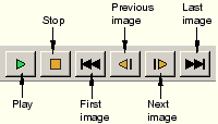
From left to right, these controls perform the following functions: play, stop, first image, previous image, next image, last image.
To change the animation control options, click Animation Options in the prompt area.
The Animation Options dialog box appears; by default, the Player tab is selected.
From the Mode option, choose Play once.
Click OK.
You will see from the animation that as the blast loading is applied, the plate begins to deflect. Over the duration of the load the plate begins to vibrate and continues to vibrate after the blast load has dropped to zero. The maximum displacement occurs at approximately 8 ms, and a displaced plot of that state is shown in Figure 5–15.
The animation images can be saved to a file for playback at a later time.
To save the animation:
From the main menu bar, select Animate![]() Save As.
Save As.
The Save Image Animation dialog box appears.
In the Settings field, enter the file name blast_base.
The format of the animation can be specified as either QuickTime or AVI.
Choose the QuickTime format, and click OK.
The animation is saved as blast_base.mov in your current directory. You can play the animation file using the ABAQUS movie player utility.
To play an animation file using the movie player:
From the main menu bar, select Animate![]() Image Animation.
Image Animation.
The Open Image Animation dialog box appears.
Select the file blast_base.mov.
Click OK.
The ABAQUS movie player utility appears, and the animation automatically starts to play.
To change any of the default options, click Animation Options in the prompt area.
After the animation has finished, click Dismiss in the prompt area to exit the ABAQUS movie player utility.
History output
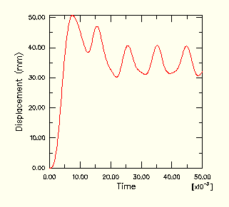
Since it is not particularly easy to see the deformation of the plate from the deformed plot, it may be better to view the deflection response of the central node (node set NOUT) in the form of a graph. The displacement of the node in the center of the plate is of particular interest since the largest deflection occurs at this node.
To generate a history plot of the central node displacement:
Use the following commands to display the displacement history of the central node, as shown in Figure 5–16 (with displacements in millimeters).
From the main menu bar, select Result![]() History Output.
History Output.
The History Output dialog box appears.
Plot the spatial displacement, U1, at node 411.
To save the current X–Y data, click Save As. Name the data DISP.
Click Dismiss.
The units of the displacements in this plot are meters. Modify the data to create a plot of displacement (in millimeters) versus time.
Select Tools![]() XY Data
XY Data![]() Manager.
Manager.
The DISP data are listed in the XY Data Manager dialog box.
To create the plot with the displacement values in millimeters, you need to multiply the DISP X–Y data by 1000.
Click Create in the XY Data Manager dialog box; then select Operate on XY Data in the Create XY Data dialog box. Click Continue.
The Operate on XY Data dialog box opens.
Click DISP in the XY Data field; then click * in the Operators field.
In the text box at the top of the dialog box, enter 1000 following the * symbol so that the expression appears as:
"DISP" * 1000
Click Plot Expression to see the modified X–Y data. Save the data as U_BASE2.
Click Cancel.
To change the plot titles, click XY Plot Options in the prompt area.
The XY Plot Options dialog box appears. Click the Titles tab.
Click Title source for the Y-axis and select User-specified. Change the title to Displacement (mm).
Click OK. The resulting plot is shown in Figure 5–16.
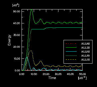
The other quantities saved as history output in the output database are the total energies of the model. The energy histories can help identify possible shortcomings in the model as well as highlight significant physical effects.
To generate history plots of the model energies:
Use the following commands to display the histories of five different energy output variables—ALLKE, ALLSE, ALLPD, ALLIE, and ALLAE.
From the main menu bar, select Result![]() History Output.
History Output.
The History Output dialog box appears.
Select the output variable Artificial strain energy: ALLAE for Whole Model. Click Save As. Name the curve ALLAE.
Click OK.
Similarly, save the history results for the ALLKE, ALLSE, ALLPD, and ALLIE output variables as X–Y data.
Click Dismiss.
Select Tools![]() XY Data
XY Data![]() Manager.
Manager.
The ALLAE, ALLKE, ALLSE, ALLPD, and ALLIE X–Y data objects are listed in the XY Data Manager.
In the XY Data Manager dialog box, select ALLAE, ALLKE, ALLSE, ALLPD, and ALLIE using [Ctrl]+Click; and click Plot to plot the energy curves.
Click Dismiss.
To more clearly distinguish between the different curves in the plot, change their line styles.
Click XY Curve Options in the prompt area.
The XY Curve Options dialog box appears.
For the curve ALLSE, select a dashed line style and click Apply.
For the curve ALLPD, select a dotted line style and click Apply.
For the curve ALLAE, select a chain dashed line style and click Apply.
For the curve ALLIE, select the second thinnest line type and click Apply.
Click Dismiss.
Customize the appearance of the plot further by changing the plot titles and the position of the legend.
To change the plot titles, click XY Plot Options in the prompt area.
The XY Plot Options dialog box appears. Click the Titles tab.
Change the title for the Y-axis to Energy.
Click OK.
To change the position of the legend, select Viewport![]() Viewport Annotation Options.
Viewport Annotation Options.
Click the Legend tab.
The position of the upper left corner of the legend is determined by the values specified in the % Viewport X and % Viewport Y boxes.
Change the % Viewport X value to 65, and the % Viewport Y value to 50.
This will position the legend so that the upper left corner is 65% of the way across the viewport from left to right and 50% of the way up the viewport from bottom to top.
Click OK. The resulting plot is shown in Figure 5–17.
We can see that once the load has been removed and the plate vibrates freely, the kinetic energy increases as the strain energy decreases. When the plate is at its maximum deflection and, therefore, has its maximum strain energy, it is almost entirely at rest, causing the kinetic energy to be at a minimum.
Note that the plastic strain energy rises to a plateau and then rises again. From the plot of kinetic energy we can see that the second rise in plastic strain energy occurs when the plate has rebounded from its maximum displacement and is moving back in the opposite direction. We are, therefore, seeing plastic deformation on the rebound after the blast pulse.
Even though there is no indication that hourglassing is a problem in this analysis, study the artificial strain energy to make sure. As discussed in Chapter 4, “Finite Elements and Rigid Bodies,” artificial strain energy is the energy used to control hourglass deformation, and the output variable ALLAE is the accumulated artificial strain energy. Since energy is dissipated as plastic deformation as the plate deforms, the total internal energy is much greater than the elastic strain energy alone. Therefore, it is most meaningful in this analysis to compare the artificial strain energy to an energy quantity that includes the dissipated energy as well as the elastic strain energy. Such a variable is the total internal energy, ALLIE, which is a summation of all internal energy quantities. The artificial strain energy is approximately 1% of the total internal energy, indicating that hourglassing is not a problem.
One thing we can notice from the deformed shape is that the central stiffener is subject to almost pure in-plane bending. Using only two first-order, reduced-integration elements through the depth of the stiffener is not sufficient to model in-plane bending behavior. While the solution from this coarse mesh appears to be adequate since there is little hourglassing, for completeness we will study how the solution changes when we refine the mesh of the stiffener. Remember that caution must be taken when refining the mesh, since mesh refinement will increase the solution time by increasing the number of elements and decreasing the element size.
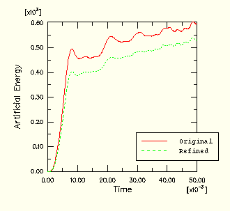
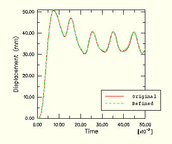
An input file for a model with a refined stiffener mesh is included in “Blast loading on a stiffened plate,” Section A.5 (blast_refined.inp); four elements through the depth are used to model the stiffener instead of two. This increase in the number of elements increases the solution time by approximately 20%. In addition, the stable time increment decreases by approximately a factor of two as a result of the reduction of the smallest element dimension in the stiffeners. Since the total increase in solution time is a combination of the two effects, the solution time of the refined mesh increases by approximately a factor of 1.2 × 2, or 2.4, over that of the original mesh.
Figure 5–18 shows the histories of artificial energy for both the original mesh and the mesh with the refined stiffeners. As anticipated, the artificial energy is lower in the refined mesh. The important question, however, is whether or not the results changed significantly from the original to the refined mesh. Figure 5–19 shows that the displacement of the plate's central node is almost identical in both cases, indicating that the original mesh is capturing the overall response adequately. One advantage of the refined mesh, however, is that it better captures the variation of stress and plastic strain through the stiffeners.
Contour plots
Use the contour plotting capability of ABAQUS/Viewer to display the von Mises stress and equivalent plastic strain distributions in the plate. Use the model with the refined stiffener mesh to create the plots: from the main menu bar, select File![]() Open and choose the file blast_refined.odb.
Open and choose the file blast_refined.odb.
To generate contour plots of the von Mises stress and equivalent plastic strain:
From the main menu bar, select Result![]() Field Output.
Field Output.
The Field Output dialog box appears.
Select the stress output variable (S) from the Output Variable area. The stress invariants are displayed in the Invariant area.
Select the Mises stress invariant.
Click Section Points to select a section point.
The Section Points dialog box appears.
Select shell under Category and the SPOS section point from the list of available section points.
Click OK.
The Select Plot Mode dialog box appears.
Toggle on Contour, and click OK.
ABAQUS/Viewer displays a contour plot of the von Mises stress.
The view that you set earlier for the animation exercise should be changed so that the stress distribution is clearer. By default, only feature edges are visible. Change this so that all element edges are visible. You will also need to reposition the legend in the plot.
From the main menu bar, select View![]() Views Toolbox to bring up the Views dialog box. Select the isometric view.
Views Toolbox to bring up the Views dialog box. Select the isometric view.
To show all the visible edges, click Contour Options in the prompt area.
The Contour Plot Options dialog box appears.
Choose Exterior visible edges.
Click OK.
To change the legend position back to the default position, select Viewport![]() Viewport Annotation Options from the main menu bar.
Viewport Annotation Options from the main menu bar.
Click the Legend tab in the Viewport Annotation Options dialog box. Click Defaults to reset the legend position to its default location.
Click OK.
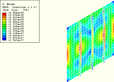
Figure 5–20 shows a contour plot of the von Mises stress at the SPOS section point (section point 5).
Now contour the equivalent plastic strain.
From the main menu bar, select Result![]() Field Output.
Field Output.
The Field Output dialog box appears.
Select the equivalent plastic strain output variable (PEEQ) from the Output Variable area.
Click OK.
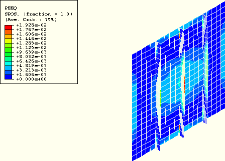
Figure 5–21 shows a contour plot of the equivalent plastic strain at the SPOS section point (section point 5).
The objective of this analysis is to study the deformation of the plate and the stress in various parts of the structure when it is subjected to a blast load. To judge the accuracy of the analysis, you will need to consider the assumptions and approximations made and identify some of the limitations of the model.
Damping
Undamped structures continue to vibrate with constant amplitude. Over the 50 ms of this simulation the frequency of the oscillation can be seen to be approximately 214 Hz. A constant amplitude vibration is not the response that would be expected in practice since the vibrations in this type of structure would tend to die out over time and effectively disappear after 5–10 oscillations. The energy loss typically occurs by a variety of mechanisms including frictional effects at the supports and damping by the air.
Consequently, we need to consider the presence of damping in the analysis to model this energy loss. The energy dissipated by viscous effects, ALLVD, is nonzero, indicating that there is already some damping present in the analysis. By default, a bulk viscosity damping (discussed in Chapter 3, “Overview of Explicit Dynamics”) is always present and is introduced to improve the modeling of high-speed events.
In this shell model only linear damping is present. With the default value the oscillations would eventually die away, but it would take a long time because the bulk viscosity damping is very small. Material damping should be used to introduce a more realistic structural response. Modify the material data block to include damping, setting the mass proportional damping to 50.0.
*DAMPING, ALPHA=50.0, BETA=0.0BETA is the parameter that controls stiffness proportional damping, and at this stage we will leave it set to zero.
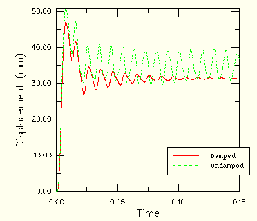
The time period for the oscillation of the plate is approximately 10 ms, so we need to increase the analysis period to allow enough time for the vibration to be damped out. Therefore, increase the analysis period to 150 ms.
The results of the damped analysis clearly show the effect of mass proportional damping. Figure 5–22 shows the displacement history of the central node for both the damped and undamped analyses. (We have extended the analysis time to 150 ms for the undamped model to compare the data more effectively.) The peak response is also reduced due to damping. By the end of the damped analysis the oscillation has decayed to a nearly static condition.
Rate dependence
Some materials, such as mild steel, show an increase in the yield stress with increasing strain rate. In this example the loading rate is high, so strain-rate dependence is likely to be important. The *RATE DEPENDENT option is used with the *PLASTIC option to introduce strain-rate dependence.
Add the following to the material option block:
*RATE DEPENDENT
40.0, 5.0
With this definition of rate-dependent behavior, the ratio of the dynamic yield stress to the static yield stress (
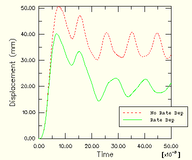
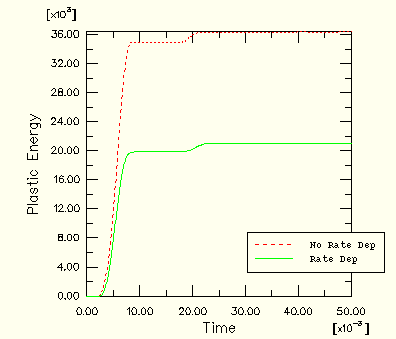
When the *RATE DEPENDENT option is included, the yield stress effectively increases as the strain rate increases. Therefore, because the elastic modulus is higher than the plastic modulus, we expect a stiffer response in the analysis with rate dependence. Both the displacement history of the central portion of the plate shown in Figure 5–23 and the history of plastic strain shown in Figure 5–24 confirm that the response is indeed stiffer when rate dependence is included.
The results are, of course, sensitive to the material data. In this case the values of