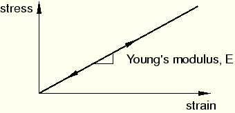
Many metals exhibit approximately linear elastic behavior at low strain levels, as shown in Figure 5–1.
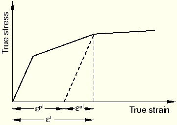
A constant stiffness, called the Young's modulus or the elastic modulus, characterizes the material behavior. At higher strain levels metals exhibit nonlinear, plastic behavior, as shown in Figure 5–2.The plastic behavior of a material is described by its yield point and its post-yield hardening. Figure 5–2 shows a stress-strain curve for a ductile metal with all the important regions labeled. At a point on the stress-strain curve known as the elastic limit or the yield point, the behavior changes from elastic to plastic. In most metals the stress at the yield point, called the yield stress, is 0.05 to 0.1% of the material's elastic modulus.
The deformation of the metal prior to reaching the yield point creates only elastic strains, which are recovered fully if the applied load is removed. However, once the stress in the metal exceeds the yield stress, permanent or plastic deformation begins to occur. Strains associated with plastic deformation are called plastic strains. Even after yielding, the elastic strains continue to increase according to the original elastic modulus, so that any additional straining contains both elastic and plastic components.
Once the metal yields, the stiffness for continued loading decreases dramatically, while the Young's modulus still defines the stiffness when unloading. If the material is loaded again after unloading, its stiffness is equal to the Young's modulus until its stress-strain curve on reloading once again intersects the hardening curve, at which point the material yields and continues loading along the hardening curve. Often plastic deformation increases a material's yield stress upon subsequent loadings, a behavior called work hardening.
A metal deforming plastically under a tensile load may experience highly localized deformation, called necking, after reaching its ultimate strength. During necking the nominal stress (force per unit original area) drops well below the ultimate strength, as the nominal strain (length change per unit original length) continues to increase. This material behavior is caused by the geometry of the test specimen, the nature of the test itself, and the stress and strain measures used. For example, testing the same material in compression produces a stress-strain curve that does not have a necking region because the specimen does not thin as it deforms in compression. A mathematical model describing the plastic behavior of metals must be able to account for differences in the compressive and tensile behavior independent of the structure's geometry or the nature of the applied loads. Replacing nominal stress, ![]() , and nominal strain,
, and nominal strain, ![]() , with alternative stress and strain measures allows us to account for the change in area during the finite deformations.
, with alternative stress and strain measures allows us to account for the change in area during the finite deformations.
Strains in compression and tension are the same only if considered in the limit as ![]() ; i.e.,
; i.e.,
![]()
![]()
The stress measure that is the conjugate to the true strain is called the true stress and is defined as
![]()
When defining plasticity data in ABAQUS, you must use true stress and true strain. ABAQUS requires these values to interpret the data in the input file correctly. However, quite often material test data are supplied using values of nominal stress and strain. In such situations you must convert the plastic material data from nominal stress and strain to true stress and strain.
The relationship between true strain and nominal strain is established by expressing the nominal strain as
![]()
![]()
The relationship between true stress and nominal stress is formed by considering the incompressible nature of the plastic deformation and assuming the elastic volumetric deformation is negligible, so
![]()
![]()
![]()
![]()
![]()
![]()
Use the *PLASTIC option in ABAQUS to define the post-yield behavior for most metals. The data pairs on the *PLASTIC option define the true stress as a function of true plastic strain. The first data pair defines the initial yield stress and the corresponding initial plastic strain, which must have a value of zero. ABAQUS connects your stress-strain data pairs with a series of straight line segments to form a continuous, piecewise-linear plasticity curve. You can use any number of data pairs to approximate the actual material behavior; therefore, it is possible to get a very close approximation to the actual material behavior.
The strains provided in material test data used to define the plastic behavior are not likely to be the plastic strains in the material. Instead, they will probably be the total strains in the material. You must decompose these total strain values into the elastic and plastic strain components. The plastic strain is obtained by subtracting the elastic strain, defined as the value of true stress divided by the Young's modulus, from the value of total strain (see Figure 5–3). This relationship is written
![]()
![]()
is true plastic strain,
![]()
is true total strain,
![]()
is true elastic strain,
![]()
is true stress, and
![]()
Example of converting material test data to ABAQUS input
The stress-strain curve in Figure 5–4 will be used as an example of how to convert the test data defining a material's plastic behavior into the appropriate input format for ABAQUS. The six points shown on the nominal stress-strain curve will be used as the data for the *PLASTIC option.
The first step is to use the equations relating the true stress to the nominal stress and strain and the true strain to the nominal strain to convert the nominal stress and nominal strain to true stress and true strain. Once these values are known, the equation relating the plastic strain to the total and elastic strains (shown earlier) can be used to determine the plastic strains associated with each yield stress value. The converted data are shown in Table 5–1.
Table 5–1 Converting nominal stress and strain to true stress and strain.
| Nominal Stress | Nominal Strain | True Stress | True Strain | Plastic Strain |
|---|---|---|---|---|
| 200E6 | 0.00095 | 200.2E6 | 0.00095 | 0.0 |
| 240E6 | 0.025 | 246E6 | 0.0247 | 0.0235 |
| 280E6 | 0.050 | 294E6 | 0.0488 | 0.0474 |
| 340E6 | 0.100 | 374E6 | 0.0953 | 0.0935 |
| 380E6 | 0.150 | 437E6 | 0.1398 | 0.1377 |
| 400E6 | 0.200 | 480E6 | 0.1823 | 0.1800 |
Regularization of user-defined data
When performing an analysis, ABAQUS/Explicit may not use exactly the material data defined by the user; for efficiency, all material data that are defined in tabular form are automatically regularized. Material data can be functions of temperature, external fields, and internal state variables, such as plastic strain. For each material point calculation, the state of the material must be determined by interpolation, and, for efficiency, ABAQUS/Explicit fits the user-defined curves with curves composed of equally spaced points. These regularized material curves are the material data used during the analysis. It is important to understand the differences that might exist between the regularized material curves used in the analysis and the curves that you specified in your input file.
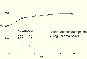
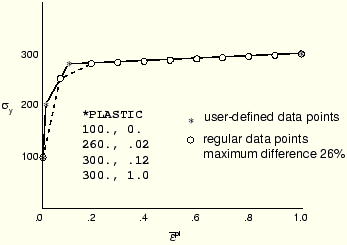
To illustrate the implications of using regularized material data, consider the following two cases. Figure 5–5 shows a case in which the user has defined data that are not regular. In this example ABAQUS/Explicit generates the six regular data points shown, and the user's data are reproduced exactly. Figure 5–6 shows a case where the user has defined data that are difficult to regularize exactly. In this example it is assumed that ABAQUS/Explicit has regularized the data by dividing the range into 10 intervals that do not reproduce the user's data points exactly.
ABAQUS/Explicit attempts to use enough intervals such that the maximum error between the regularized data and the user-defined data is less than 3%. You can change this error tolerance by using the RTOL parameter on the *MATERIAL option. If more than 200 intervals are required to obtain an acceptable regularized curve, the analysis stops during the data checking with an error message. In general, the regularization is more difficult if the smallest interval defined by the user is small compared to the range of the independent variable. In Figure 5–6 the data point for a strain of 1.0 makes the range of strain values large compared to the small intervals defined at low strain levels. Removing this last data point enables the data to be regularized much more easily.
Interpolation between data points
ABAQUS/Explicit interpolates linearly between the regularized data points to obtain the material's response and assumes that the response is constant outside the range defined by the input data. Thus, the stress in the material shown in Figure 5–5 and Figure 5–6 will never exceed 300 MPa; when the stress in the material reaches 300 MPa, the slope of the hardening curve is assumed to be zero.