This simulation of the forming of a channel in a long metal sheet illustrates the use of rigid surfaces and some of the more complex techniques often required for a successful contact analysis.
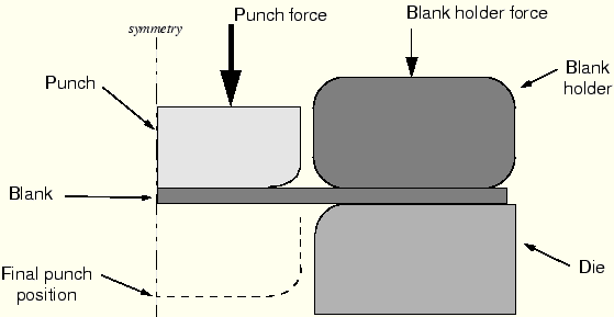
The problem consists of a strip of deformable material, called the blank, and the tools—the punch, die, and blank holder—that contact the blank. The tools can be modeled as rigid surfaces because they are much stiffer than the blank. Figure 11–19 shows the basic arrangement of the components.
The blank is 1 mm thick and is squeezed between the blank holder and the die. The blank holder force is 440 kN. This force, in conjunction with the friction between the blank and blank holder and the blank and die, controls how the blank material is drawn into the die during the forming process. You have been asked to determine the forces acting on the punch during the forming process. You also must assess how well the channel is formed with these particular settings for the blank holder force and the coefficient of friction between the tools and blank.A two-dimensional, plane strain model will be used. The assumption that there is no strain in the out-of-plane direction of the model is valid if the structure is long in this direction. Only half of the channel needs to be modeled because the forming process is symmetric about a plane along the center of the channel.
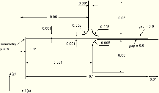
The dimensions of the various components are shown in Figure 11–20.
Two-dimensional, plane strain models are defined, by default, in the global 1–2 plane as shown in Figure 11–20. For the forming simulation, place the origin of this plane at the bottom left-hand corner of the blank (Figure 11–20). The 1-direction will be normal to the symmetry plane, which is located at ![]() .
.
The mesh for this simulation can be divided into the deformable blank and the rigid tools.
Blank
Once again, the element type should be selected before the mesh is designed. Using the selection process discussed in “Mesh design,” Section 11.4.3, incompatible mode elements are selected. The mesh used for the blank should consist of two rows of 100 CPE4I elements (see Figure 11–21). Two rows of elements are used so that better resolution of the deformation through the thickness of the blank will be obtained.
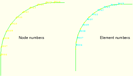
The node and element numbers for the mesh shown in Figure 11–22 are from the model of this problem given in “Forming a channel,” Section A.13. These node and element numbers are used in the discussion that follows.
Tools
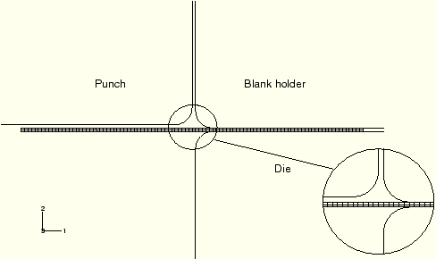
The tools are modeled with rigid surfaces. Analytical rigid surfaces are used to model the blank holder and the punch. R2D2 rigid elements are used to model the die. The mesh for the die is shown in Figure 11–23. The curved corner is modeled with 10 elements: this is done to create a sufficiently smooth surface that will capture the corner geometry accurately. Always use a sufficient number of elements to model such curves. Create three rigid body reference nodes, one for each tool. Place them roughly in the center of each tool.
Use a preprocessor to generate the mesh for the blank and the rigid die. The analytical rigid surfaces for the punch and blank holder can also be defined using a preprocessor such as ABAQUS/CAE.
If your preprocessor does not directly support rigid elements, mesh the die with 2-node beam elements such as B21. Once the ABAQUS input file has been created, change the TYPE parameter on the *ELEMENT option from B21 to R2D2, and delete any beam section options.
If you do not want to use a preprocessor, the ABAQUS input options for the model shown in Figure 11–22 and Figure 11–23 are given in “Forming a channel,” Section A.13. If you wish to create the entire model using ABAQUS/CAE please refer to “ABAQUS/Standard example: forming a channel,” Section 12.6 of Getting Started with ABAQUS.
We first review the model definition, including the node and element definitions, section and material properties, and rigid body definition.
Model description
Provide a relevant description of the simulation and model on the *HEADING option.
*HEADING
Analysis of the forming of a channel
SI units (N, kg, m, s)
Nodal coordinates and element connectivity
Check that the preprocessor used the correct element type for the blank and for the rigid elements modeling the die. Provide meaningful element set names, such as BLANK and DIE, for the two groups of elements. The *ELEMENT options in your model should look like
*ELEMENT, TYPE=CPE4I, ELSET=BLANK
*ELEMENT, TYPE=R2D2, ELSET=DIE
Create node sets so that parts of the model can be constrained and moved easily. Put the nodes that are located on the centerline of the blank and have symmetric constraints into a node set called CENTER.
*NSET, NSET=CENTER
1,102,203
Place the nodes along the middle of the blank toward the right-hand side of the model, where the blank lies between the blank holder and die, into node set MIDRIGHT.
*NSET, NSET=MIDRIGHT, GENERATE
155,202,1
Place the nodes along the middle of the sheet toward the left-hand side of the model, underneath the punch, into node set MIDLEFT.
*NSET, NSET=MIDLEFT, GENERATE
102,147,1
Again, the node numbers in these option blocks are for the model in Figure 11–22; your node numbers may be different.
These last two node sets will be used to apply temporary constraints to the blank as the simulation establishes the contact between the blank and the tools.
Define two element sets, BLANK_B and BLANK_T, containing the lower and upper rows of elements in the blank. These will be used to define the contact surfaces on the blank.
*ELSET, ELSET=BLANK_B, GENERATE
1,100,1
*ELSET, ELSET=BLANK_T, GENERATE
101,200,1
Section and material properties for the blank
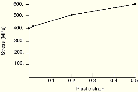
The blank is made from a high-strength steel (elastic modulus of 210.0 GPa, ![]() = 0.3). Its inelastic stress-strain behavior is shown in Figure 11–24. The material undergoes considerable work hardening as it deforms plastically. It is likely that plastic strains will be large in this analysis; therefore, hardening data are provided up to 50% plastic strain.
= 0.3). Its inelastic stress-strain behavior is shown in Figure 11–24. The material undergoes considerable work hardening as it deforms plastically. It is likely that plastic strains will be large in this analysis; therefore, hardening data are provided up to 50% plastic strain.
The blank is going to undergo significant rotation as it deforms. Reporting the values of stress and strain in a coordinate system that rotates with the blank's motion will make it much easier to interpret the results. Therefore, an *ORIENTATION option should be used to create a coordinate system that is aligned initially with the global coordinate system but moves with the elements as they deform. The following input options are needed to define the blank's element and material properties:
*SOLID SECTION,MATERIAL=STEEL,ORIENTATION=LOCAL,
 ELSET=BLANK
*ORIENTATION, NAME=LOCAL
1.,0.,0., 0.,1.,0.
3,0
*MATERIAL, NAME=STEEL
*ELASTIC
2.1E11,0.3
*PLASTIC
400.E6, 0.0E-2
420.E6, 2.0E-2
500.E6,20.0E-2
600.E6,50.0E-2
Rigid body
The R2D2 elements forming the surface of the die must be tied together to form a rigid body. To do so, specify the element set containing all of the elements on the *RIGID BODY option. Use the REF NODE parameter to assign a rigid body reference node to the elements. Add the following input to your model:
*RIGID BODY, ELSET=DIE, REF NODE=9000The values for the ELSET and REF NODE parameters reflect the model shown in “Forming a channel,” Section A.13, and may need to be changed to reflect your data. If you forgot to create a rigid body reference node for the die when building the model in the preprocessor, add the following line to your input file:
*NODE, NSET=REFDIE
9000,0.1,-0.06
The contact definitions for each part of the model are discussed here.
Rigid surfaces
The surface of the die is created from the mesh of R2D2 elements. These elements are in an element set called DIE. Specify the side of the elements that form the contact surface. The surface is on the positive side of the elements created in the model in “Forming a channel,” Section A.13, so the following input defines the surface DIE on the mesh of rigid elements:
*SURFACE, NAME=DIE
DIE, SPOS
You may have defined the rigid elements differently; check your element definitions to determine whether the surface lies on the positive or negative side of the elements.
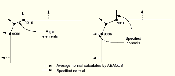
When rigid elements are used to define a rigid surface, the contact direction is determined by the nodal normal, which is the average of the normals of the elements attached to the node. Precise normals can be specified by using the *NORMAL option. This option allows you to specify the exact nodal normal that is used at a given node on a given contact surface. In this simulation use it to specify the nodal normals at nodes 9006 and 9016 to better define the contact direction. The effect of specifying the normals to the surface is illustrated in Figure 11–25. For the sake of clarity, only two elements are used to represent the corner of the die in this figure, instead of the 10 that are actually used.
Add the following option block to your input file (if necessary, change the node numbers to values appropriate for your model):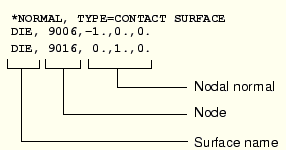
The blank holder and the punch are modeled with analytical rigid surfaces. A rigid body reference node will be assigned to each of these surfaces when they are created. If you did not create these rigid body reference nodes, add the following option block to your model:
*NODE, NSET=REFPUNCH
7000, 0.000, 0.061
*NODE, NSET=REFHOLD
8000, 0.1,0.06
Each node is placed in a node set to make the input file easy to read. While someone unfamiliar with the specific mesh used in the simulation may not know why boundary conditions are applied to node 7000, they might be able to guess why boundary conditions were applied to the REFPUNCH node.
To ensure that an analytical rigid surface's normals point toward the deformable surfaces that the rigid surface will contact, the segments composing the rigid surface must be defined in a particular order. For example, to create the correct normals for the surface PUNCH, define the surface from the top right corner to the bottom left corner of the punch. Add the following input to your model to create the surface PUNCH:
*SURFACE, TYPE=SEGMENTS, NAME=PUNCH, FILLET RADIUS=0.001
START,0.050, 0.061
LINE, 0.050, 0.007
CIRCL,0.045, 0.002, 0.045,0.007
LINE,-0.010, 0.002
*RIGID BODY, ANALYTICAL SURFACE=PUNCH, REF NODE=7000
The parameter TYPE=SEGMENTS specifies that a two-dimensional rigid surface is being defined. The NAME parameter specifies the name of the surface, PUNCH. The data lines define the geometry of the surface. The first data line always has the word “START” followed by the 1- and 2-coordinates of the starting point for the surface. The subsequent lines define line, circular, and parabolic segments. For this surface the second data line defines a straight line from the start position (0.05, 0.061) to (0.050, 0.007). The third data line defines a circular arc from the end of the straight line (0.05, 0.007) to (0.045, 0.002) with the center of the circle located at (0.045, 0.007). The last data line defines a straight line from the end of the arc to (–0.010, 0.002).
This definition should produce a smooth rigid surface but, to be safe, the FILLET RADIUS parameter specifies that a 1 mm fillet radius should be used to smooth any discontinuities in the surface definition. It is always good practice to add the FILLET RADIUS parameter to the definition of any analytical rigid surface.
The *RIGID BODY option is used to bind the analytical surface to a rigid body with its rigid body reference node specified by the REF NODE parameter and the surface referred to by its name, using the ANALYTICAL SURFACE parameter.
The rigid surface for the blank holder is defined in a similar way. Add the following option block to your model to define the surface on the blank holder:
*SURFACE, TYPE=SEGMENTS, NAME=HOLDER, FILLET RADIUS=0.001
START,0.110, 0.001
LINE, 0.056,0.001
CIRCL,0.051,0.006, 0.056,0.006
LINE, 0.051,0.060
*RIGID BODY, ANALYTICAL SURFACE=HOLDER, REF NODE=8000
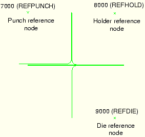
All of the rigid surfaces in this simulation extend beyond the deformable blank to ensure that there is no possibility that slave nodes will slide behind any of them. The initial configuration of these surfaces and the locations of their reference nodes are shown in Figure 11–26.
Deformable surfaces
Using the two element sets defined on the blank, create a contact surface on the top of the blank, called BLANK_T, and one on the bottom, called BLANK_B. If you use the automatic free surface generation capability, the option blocks will look like
*SURFACE, NAME=BLANK_B, TRIM=YES
BLANK_B,
*SURFACE, NAME=BLANK_T, TRIM=YES
BLANK_T,
Contact pairs
Contact must be defined between the top of the blank and the punch, the top of the blank and the blank holder, and the bottom of the blank and the die. The rigid surface must be the master surface in each of these contact pairs. Each contact pair must refer to a *SURFACE INTERACTION option that defines a surface interaction model governing how the surfaces of the contact pair interact with each other. Multiple contact pairs can refer to the same *SURFACE INTERACTION option.
In this example we assume that the friction coefficient is zero between the blank and the punch. The friction coefficient between the blank and the other two tools is assumed to be 0.1. Therefore, two *SURFACE INTERACTION options must be used in the model: one with friction and one without. Frictionless contact is the default in ABAQUS, so no *FRICTION option is needed in the surface interaction definition for the BLANK_T-PUNCH contact pair.
The option blocks to define the contact pairs and surface interactions in your model will look like
*CONTACT PAIR, INTERACTION=FRIC
BLANK_B, DIE
*CONTACT PAIR, INTERACTION=FRIC
BLANK_T, HOLDER
*CONTACT PAIR, INTERACTION=NOFRIC
BLANK_T, PUNCH
*SURFACE INTERACTION, NAME=FRIC
*FRICTION
0.1,
*SURFACE INTERACTION, NAME=NOFRIC
There are two major sources of difficulty in contact analyses: rigid body motion of the components before contact conditions constrain them and sudden changes in contact conditions, which lead to severe discontinuity iterations as ABAQUS tries to establish the exact condition of all contact surfaces. Therefore, wherever possible, take precautions to avoid these situations.
Removing rigid body motion is not particularly difficult. Simply ensure that there are enough constraints to prevent all rigid body motions of all the components in the model. This may mean using boundary conditions initially to get the components into contact, instead of applying loads directly. Using this approach may require more steps than originally anticipated, but the solution of the problem should proceed more smoothly.
Unless a dynamic impact event is being simulated, always try to establish contact between components in a reasonably smooth manner, avoiding large overclosures and rapid changes in contact pressure. Again, this usually means adding additional steps to the analysis to move components into contact before fully loading them. This approach, although requiring more steps, will minimize convergence difficulties and, therefore, make the solution far more efficient. With these points in mind, we can now design the history data for this example.
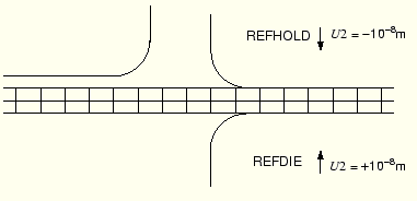
Step 1
The first stage of the process is to hold the blank between the blank holder and the die. At the start of the first increment of the analysis, contact may not be fully established between the various components, even though their surfaces are coincident initially. Problems can occur when contact is not fully established: components may undergo rigid body motion; or the contact status may oscillate between open and closed, which is known as chattering. Chattering is especially common in contact analyses with multiple components.
To avoid rigid body motions and chattering in this simulation, fix the midplane of the blank in the vertical direction to prevent the blank from moving initially. The midplane of the blank is used because constraints should not be applied to nodes that are also part of a contact surface. If a contact node is constrained by a boundary condition in the direction that contact occurs, there will be two constraints applied to a single degree of freedom. This can cause numerical problems, and ABAQUS may issue a zero pivot warning message in the message file.
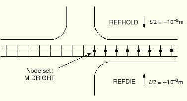
One method of establishing contact is to apply a force to the blank holder. However, the blank holder may undergo rigid body motion in the vertical direction because contact between the blank holder and the blank may not be fully established. Therefore, it is better to move the blank holder by means of an applied displacement with a *BOUNDARY option. This ensures firm contact between these two surfaces. In addition, move the die slightly upward to establish firm contact between it and the blank. The magnitude of the applied displacement is chosen large enough so that firm contact is established yet small enough so that plastic yielding does not occur. The motion of the tools in the first step, including the magnitudes, is summarized in Figure 11–27.
Constrain the blank holder and die in degrees of freedom 1 and 6, where degree of freedom 6 is the rotation in the plane of the model. All of the boundary conditions for the rigid surfaces are applied to their respective rigid body reference nodes. Constrain the punch completely, and apply symmetric boundary constraints on the nodes of the blank lying on the symmetry plane (node set CENTER).
The effects of geometric nonlinearity must be considered in this simulation, so include the NLGEOM parameter on the *STEP option. The step should complete in one increment, so on the *STATIC option set the initial time increment and the total time to be equal. To limit the amount of output, write the preselected field output only at the end of the step, and do not print any results to the data (.dat) file. Field data will be requested at a later stage in the analysis. Additionally, define a node set containing the three rigid body reference nodes, and add a request for history output of the displacements and reaction forces at these nodes. Also, use the *PRINT, CONTACT=YES option to write contact diagnostics to the message file.
The complete step definition in your model should be similar to the following:
*STEP, NLGEOM
Push the blank holder and die together
*STATIC
1.0,1.0
*BOUNDARY
MIDRIGHT,2
MIDLEFT ,2
CENTER  ,XSYMM
REFDIE  ,1
REFDIE  ,2,, 1.E-8
REFDIE  ,6
REFPUNCH,ENCASTRE
REFHOLD ,1
REFHOLD ,2,,-1.E-8
REFHOLD ,6
*PRINT, CONTACT=YES
*NODE PRINT, FREQUENCY=0
*EL PRINT, FREQUENCY=0
*OUTPUT, FIELD, FREQUENCY=0
*NSET, NSET=NOUT
REFDIE, REFHOLD, REFPUNCH
*OUTPUT, HISTORY, FREQUENCY=1
*NODE OUTPUT, NSET=NOUT
RF,U
*END STEP
Step 2
Step 1 established contact between the blank and the blank holder and die, which fully constrains the blank in the 2-direction. Therefore, the boundary conditions on the right half of the midplane of the blank (node set MIDRIGHT) can now be removed, as shown in Figure 11–28. Remove the boundary constraints by using the OP=NEW parameter on the *BOUNDARY option; however, you must respecify all of the constraints that remain in effect.
This step should also complete in a single increment because the only change being made to the model is the removal of the vertical constraints on the blank; therefore, set the initial time increment and the total time to be equal. The output requests do not need to be changed. The input data defining the second step are, therefore,
*STEP, NLGEOM
Remove the middle constraint
*STATIC
1.0,1.0
*BOUNDARY, OP=NEW
MIDLEFT ,2
CENTER  ,XSYMM
REFDIE  ,1
REFDIE  ,2,, 1.E-8
REFDIE  ,6
REFPUNCH,ENCASTRE
REFHOLD ,1
REFHOLD ,2,,-1.E-8
REFHOLD ,6
*END STEP
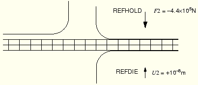
Step 3
The magnitude of the blank holder force is a controlling factor in many forming processes; therefore, it needs to be introduced as a variable load in the analysis. In Step 3 remove the boundary condition used to move the blank holder down and replace it with a force specified using a *CLOAD option, as shown in Figure 11–29.
There should be no problems replacing the applied displacement on the blank holder with a force because there is firm contact between the blank holder and the blank. In this simulation the required blank holder force is 440 kN. Generally, care should be taken to ensure that the newly applied force is of the same order as the reaction force generated from the boundary condition so that the contact condition does not change significantly.Again, use the OP=NEW parameter on the *BOUNDARY option to remove the constraint on the blank holder in degree of freedom 2, and respecify the remaining boundary conditions. This step will also complete in a single increment, so set the initial time increment to be equal to the total time. The output requests do not need to be changed.
The input for Step 3 is
*STEP, NLGEOM
Apply prescribed force on blank holder
*STATIC
1.0,1.0
*BOUNDARY, OP=NEW
MIDLEFT ,2
CENTER  ,XSYMM
REFDIE  ,1
REFDIE  ,2,, 1.E-8
REFDIE  ,6
REFPUNCH,ENCASTRE
REFHOLD ,1
REFHOLD ,6
*CLOAD
REFHOLD,2,-4.4E5
*END STEP
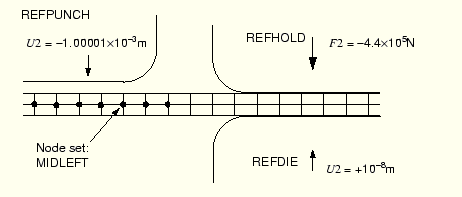
Step 4
At the beginning of the analysis the punch and the blank are separated to avoid any interference while contact is established between the blank and the die and blank holder. In this step the punch is moved down in the 2-direction just enough to achieve contact with the blank, as shown in Figure 11–30.
The vertical constraint on node set MIDLEFT is removed, and a small pressure is applied to the surface of the elements in element set BLANK_T to pull them onto the surface of the punch. It can be difficult to choose the proper magnitude of pressure to apply. In this analysis we will pick a pressure magnitude (1000 Pa) that produces a force on the blank that is three orders of magnitude lower than the blank holder force. A positive pressure acts into the surface; however, in this simulation we want the pressure to act out of the surface, so use a negative pressure. This technique is used to prevent chattering of the BLANK_T and PUNCH surfaces. Leave the output requests unchanged in this step.Set the initial time increment to 10% of the total time since the contact condition may be harder to establish in this step. The following input options should be used for Step 4:
*STEP, NLGEOM
Move the punch down a little while applying a small
pressure to BLANK_T
*STATIC
0.1,1.0
*BOUNDARY, OP=NEW
CENTER  ,XSYMM
REFDIE  ,1
REFDIE  ,2,, 1.E-8
REFDIE  ,6
REFPUNCH,1
REFPUNCH,2,,-1.000001E-3
REFPUNCH,6
REFHOLD ,1
REFHOLD ,6
*DLOAD
BLANK_T, P3, -1000.0E0
*END STEP
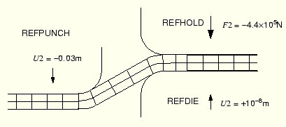
Step 5
Remove the pressure load applied to element set BLANK_T and move the punch down to complete the forming operation, as shown in Figure 11–31. When a pressure load is removed in a static analysis, the magnitude is ramped down to zero over the duration of the step. Therefore, the pressure will continue to pull on the surface BLANK_T and hold it tightly against the punch, maintaining contact between the surfaces, particularly in the early part of the step. This helps prevent chattering between the punch and the blank at the beginning of the forming process. As long as the force created by the pressure is small compared to the force required to move the punch, it will have little effect on the solution.
Between the frictional sliding, the changing contact conditions, and the inelastic material behavior, there is significant nonlinearity in this step; therefore, set the maximum number of increments to a large value (for example, set INC=1000 on the *STEP option). Also, set the initial time increment to be 0.0001, the total step time to be 1.0, and the minimum time increment to be 10–6. Therefore, ABAQUS can take smaller time increments during the highly nonlinear parts of the response without terminating the analysis.
In this step field output will be requested at the end of the step. The previous history output requests remain in effect because the OP parameter is set to ADD on the *OUTPUT option. The input for Step 5 is
*STEP, INC=1000, NLGEOM
Move the punch down to full extent
*STATIC
.0001,1.0,1.E-6
*BOUNDARY
CENTER  ,XSYMM
REFDIE  ,1
REFDIE  ,2,, 1.E-8
REFDIE  ,6
REFPUNCH,1
REFPUNCH,2,,-0.03
REFPUNCH,6
REFHOLD ,1
REFHOLD ,6
*DLOAD, OP=NEW
*OUTPUT, FIELD, FREQ=1000, OP=ADD
*ELEMENT OUTPUT, ELSET=BLANK
 S, PE, PEEQ
*NODE OUTPUT
 U
*CONTACT OUTPUT,MASTER=PUNCH
 CSTRESS
*END STEP
Contact analyses are generally more difficult to complete than just about any other type of simulation in ABAQUS. Therefore, it is important to understand all of the options available to help you with contact analyses.
If a contact analysis runs into difficulty, the first thing to check is whether the contact surfaces are defined correctly. The easiest way to do this is to run a datacheck analysis and plot the surface normals in ABAQUS/Viewer. You can plot all of the normals, for both surfaces and structural elements, on either the deformed or the undeformed plots. Use the Normals options in the Undeformed Shape Plot Options and Deformed Shape Plot Options dialog boxes to do this, and confirm that the surface normals are in the correct directions.
ABAQUS may still have some problems with contact simulations, even when the contact surfaces are all defined correctly. One reason for these problems may be the default convergence tolerances and limits on the number of iterations: they are quite rigorous. In contact analyses it is sometimes better to allow ABAQUS to iterate a few more times rather than abandon the increment and try again. This is why ABAQUS makes the distinction between severe discontinuity iterations and equilibrium iterations during the simulation.
The *PRINT, CONTACT=YES option is essential for almost every contact analysis. The information this option provides in the message file can be vital for spotting mistakes or problems. For example, chattering can be spotted because the same slave node will be seen to be involved in all of the severe discontinuity iterations. If you see this, you will have to modify the mesh in the region around that node or add constraints to the model. Contact data in the message file can also identify regions where only a single slave node is interacting with a surface. This is a very unstable situation and can cause convergence problems. Again, you should modify the model to increase the number of elements in such regions.
Save the input in the file channel.inp (see “Forming a channel,” Section A.13). Run the analysis in the background since it will take several minutes to an hour to complete.
abaqus job=channelCheck the status and message files while the job is running to see how it is progressing.
Status file
This analysis should take over 200 increments to complete. The top of the status file is shown below.
 SUMMARY OF JOB INFORMATION:
 STEP  INC ATT SEVERE EQUIL TOTAL  TOTAL      STEP       INC OF       DOF    IF
               DISCON ITERS ITERS  TIME/    TIME/LPF    TIME/LPF    MONITOR RIKS
               ITERS               FREQ
   1     1   1     0     2     2  1.00       1.00       1.000
   2     1   1     0     1     1  2.00       1.00       1.000
   3     1   1     0     2     2  3.00       1.00       1.000
   4     1   1     0     2     2  3.10       0.100      0.1000
   4     2   1     0     1     1  3.20       0.200      0.1000
   4     3   1     0     1     1  3.35       0.350      0.1500
   4     4   1     0     1     1  3.58       0.575      0.2250
   4     5   1     0     1     1  3.91       0.913      0.3375
   4     6   1     3     1     4  4.00       1.00       0.08750
   5     1   4     8     1     9  4.00       1.56e-06   1.563e-06
   5     2   1     3     1     4  4.00       3.13e-06   1.563e-06
ABAQUS has a very difficult time determining the contact state in the first increment of Step 5. It needs four attempts before it finds the proper configuration of the PUNCH and BLANK_T surfaces. Once it finds the correct configuration, ABAQUS only needs a single iteration to achieve equilibrium. After this difficult start, ABAQUS quickly increases the increment size to a more reasonable value. The end of the status file is shown below.5 456 1 0 2 2 4.99 0.990 0.0003959 5 457 1 0 1 1 4.99 0.991 0.0005938 5 458 1 0 1 1 4.99 0.991 0.0008907 5 459 1 0 2 2 4.99 0.993 0.001336 5 460 2 1 3 4 4.99 0.993 0.0005010 5 461 1 0 1 1 4.99 0.994 0.0007515 5 462 1 0 3 3 5.00 0.995 0.001127 5 463 1 0 2 2 5.00 0.997 0.001691 5 464 1 1 4 5 5.00 0.999 0.002536 5 465 1 1 3 4 5.00 1.00 0.0006165
This simulation, unlike the previous one, contains many severe discontinuity iterations. The message file will be quite large because of the number of iterations in the analysis. Although it might be tempting to limit the information written to this file, generally this should not be done because this information is the main source of diagnostic data that ABAQUS provides during the simulation.
Because of the length of this simulation, no printed output was requested. All results will be studied using an interactive postprocessor. Use the following command to run ABAQUS/Viewer:
abaqus viewer odb=channelat the operating system prompt.
Deformed model shape and contour plots
The basic result of this simulation is the deformation of the blank and the plastic strain caused by the forming process. We can plot the deformed model shape and the plastic strain using ABAQUS/Viewer, as described below.
To plot the deformed model shape:
From the main menu bar, select Plot![]() Deformed Shape; or click the
Deformed Shape; or click the ![]() tool in the toolbox.
tool in the toolbox.
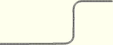
The deformed model shape at the end of Step 5 is plotted. You can remove the die and the punch from the display and visualize just the blank.
From the main menu bar, select Tools![]() Display Group
Display Group![]() Create.
Create.
The Create Display Group dialog box appears.
Select the element set PART-1-1.BLANK from the list of available element sets, and click ![]() to replace the current display group with the specified element set. Click
to replace the current display group with the specified element set. Click ![]() , if necessary, to fit the model in the viewport.
, if necessary, to fit the model in the viewport.
Click Deformed Shape Plot Options in the prompt area.
The Deformed Shape Plot Options dialog box appears.
Set the render style to Shaded.
Click OK to apply the settings and to close the dialog box. The resulting plot is shown in Figure 11–32.
To plot the contours of equivalent plastic strain:
From the main menu bar, select Plot![]() Contours; or click the
Contours; or click the ![]() tool from the toolbox to display contours of Mises stress.
tool from the toolbox to display contours of Mises stress.
Click Contour Options in the prompt area.
The Contour Plot Options dialog box appears.
Set the render style to Shaded.
Click OK to apply these settings.
From the main menu bar, select Result![]() Field Output.
Field Output.
The Field Output dialog box appears.
Select PEEQ from the Output Variable list.
PEEQ is an integrated measure of plastic strain. A non-integrated measure of plastic strain is PEMAG. PEEQ and PEMAG are equal for proportional loading.
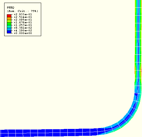
Click OK to apply these settings. Use the ![]() tool to zoom into any region of interest in the blank, as shown in Figure 11–33.
tool to zoom into any region of interest in the blank, as shown in Figure 11–33.
The maximum plastic strain is 29.3%. Compare this with the failure strain of the material to determine if the material will tear during the forming process.
History plots of the reaction forces on the blank and punch
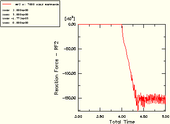
It is important to check that the force required to push the punch into the blank is much larger than the force created by the pressure applied to the surface of the blank. The force on the blank from the applied pressure is approximately 100 N (1000 Pa × 0.1 m × 1.0 m) at the start of Step 5. The solid line in Figure 11–34 shows the variation of the reaction force RF2 at the punch's rigid body reference node.
To create a history plot of the reaction force:
From the main menu bar, select Plot![]() History Output.
History Output.
A history plot of the reaction force in the 1-direction appears.
From the main menu bar, select Results![]() History Output.
History Output.
The History Output dialog box appears.
From the list of available variables, select Reaction force: RF2 at Node 7000 in NSET NOUT.
Click Plot to create a history plot of RF2.
Click Dismiss to close the dialog box.
To label the axes, click XY Plot Options in the prompt area.
The XY Plot Options dialog box appears.
Click the Titles tab, and select User-specified from the Title source pull-down lists for the X-Axis and Y-Axis labels.
Specify Reaction Force - RF2 as the Y-Axis label, and specify Total Time as the X-Axis label.
Click OK to apply the settings and to close the dialog box.
The punch force, shown in Figure 11–34, rapidly increases to about 150 kN during Step 5, which runs from a total time of 4.0 to 5.0. The punch force clearly is much larger than the force (100 N) created by the pressure load.
Plotting contours on surfaces
ABAQUS/Viewer includes a number of features designed specifically for postprocessing contact analyses. Within ABAQUS/Viewer, the Display Group feature can be used to collect surfaces into display groups, similar to element and node sets.
To display contact surface normal vectors:
From the main menu bar, select Plot![]() Undeformed Shape; or click
Undeformed Shape; or click ![]() in the toolbox to plot the undeformed model shape.
in the toolbox to plot the undeformed model shape.
From the main menu bar, select Tools![]() Display Group
Display Group![]() Create; or click
Create; or click ![]() in the toolbox.
in the toolbox.
The Create Display Group dialog box appears.
Select the surfaces BLANK_T and PUNCH from the list of available surfaces, and click ![]() to replace the current display group with the specified surfaces.
to replace the current display group with the specified surfaces.
In the prompt area, click Undeformed Shape Plot Options.
The Undeformed Shape Plot Options dialog box appears.
Click the Normals tab, toggle on Show normals, and select On surfaces to turn on the display of the normal vectors.
In the Style section, set Length to Short.
Click OK to apply the settings and to close the dialog box.
Use the ![]() tool, if necessary, to zoom into any region of interest, as shown in Figure 11–35.
tool, if necessary, to zoom into any region of interest, as shown in Figure 11–35.
To contour the contact pressure:
From the main menu bar, select Plot![]() Contours; or click
Contours; or click ![]() in the toolbox to plot the contours of plastic strain again.
in the toolbox to plot the contours of plastic strain again.
From the main menu bar, select Tools![]() Display Group
Display Group![]() Create.
Create.
The Create Display Group dialog box appears.
Select the surface PUNCH from the list of available surfaces, and click ![]() to remove the surface from the current display group.
to remove the surface from the current display group.
Now the surface BLANK_T is the only member of the display group.
From the main menu bar, select Result![]() Field Output.
Field Output.
The Field Output dialog box appears.
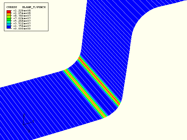
Select CPRESS from the Output Variable list.
Click OK to apply these settings.
To better visualize contours of surface-based variables in two-dimensional models, extrude the plane strain elements to construct the equivalent three-dimensional view. You can sweep axisymmetric elements in a similar fashion.
From the main menu bar, select View![]() ODB Display Options.
ODB Display Options.
The ODB Display Options dialog box appears.
Select the Sweep & Extrude tab to access the Sweep & Extrude options.
In the Extrude region of the dialog box, toggle on Extrude elements; and set the Depth to 0.05 to extrude the model for the purpose of displaying contours.
Click OK to apply these settings.
Rotate the model using the ![]() tool to display the model from a suitable view, such as the one shown in Figure 11–36.
tool to display the model from a suitable view, such as the one shown in Figure 11–36.