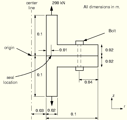
In this example you will investigate the behavior of a preliminary design for the flanged joint shown in Figure 11–10. The top flange is made from steel and the bottom flange from aluminum. The joint carries an axial load of 200 kN. An O-ring will be used to help seal the joint. In the preliminary design the O-ring will be placed 0.01 m from the inside of the flange.
You have been asked to determine the distance that the flanges separate at the seal position so that an appropriately sized seal can be selected. You should also use the computational model to confirm that the overall sizing of the flange is adequate.There appears to be no need for boundary conditions in this simulation. The forces applied to each flange are supposed to be equal in magnitude and opposite in direction; thus, the loading should be self-equilibrating. However, with no boundary conditions, there will be some small out-of-balance net force acting on the model due to the finite precision of computers. If the model is used in a static simulation with no boundary conditions (only applied forces), this small net force would cause unlimited rigid body motion of the model.
Such rigid body motion is known mathematically as a numerical singularity. When ABAQUS detects numerical singularities in a simulation, it prints a solver problem message in the message file. Such messages have the following format:
***WARNING:  SOLVER  PROBLEM.	NUMERICAL  SINGULARITY  WHEN PROCESSING NODE 302
	           D.O.F. 2 RATIO = 1.14541E+14
The node whose node number is printed in the message lies in that portion of the mesh that is unconstrained. The degree of freedom indicates the direction in which rigid body motion can occur.
Generally the results of a simulation containing numerical singularities should not be accepted as valid. To prevent numerical singularities in a static analysis, you must provide enough boundary conditions to prevent all rigid body motions of each component in the model. Rigid body motions can consist of both translations and rotations of the components. The potential rigid body motions depend on the dimensionality of the model.
| Dimensionality | Possible Rigid Body Motion |
| Three-dimensional | Translation in the 1-, 2-, and 3-directions. |
| Rotation about the 1-, 2-, and 3-axes. | |
| Axisymmetric | Translation in the 2-direction. |
| Rotation about the 3-axis (axisymmetric rigid bodies only). | |
| Plane stress | Translation in the 1- and 2-directions. |
| Plane strain | Rotation about the 3-axis. |
The flanges need to be constrained axially (the z-direction or the global 2-direction) to prevent rigid body motion during the simulation. Because the flanges are bolted together, only a single node in the model needs a boundary condition in the axial direction. The applied loading in this simulation will cause the reaction force at the constrained node to be approximately zero; therefore, the boundary condition can be applied to almost any node in the model.
Use the default axisymmetric coordinate system for this analysis. The global 1-axis is the radial direction, and the global 2-axis is the axis of symmetry in the model. The location of the origin for the model should be at the juncture of the two flanges as shown in Figure 11–10.
You should consider the type of element you will use before you design your mesh. When choosing an element type, you must consider several aspects of your model such as the model's geometry, the type of deformation that will be seen, the loads being applied, etc. The following are the important points to consider in this simulation:
The contact between the flanges. Whenever possible, first-order elements (with the exception of tetrahedral elements) should be used for contact simulations. When using tetrahedral elements, modified second-order tetrahedral elements should be used for contact simulations.
Significant bending of the flanges is expected under the applied loading. Fully integrated first-order elements exhibit shear locking when subjected to bending deformation. Therefore, either reduced-integration or incompatible mode elements should be used.
The mesh can use regularly shaped elements so the sensitivity of incompatible mode elements to distortion will not be a problem.
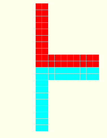
The mesh in your model should be the same as the mesh shown in Figure 11–11 because nodes are required at specific locations to represent the bolts and O-ring in the physical structure. The bolts will be modeled by a connection that extends 360 degrees.
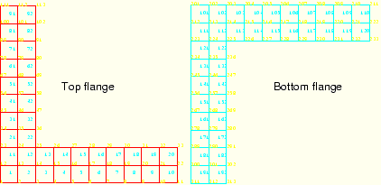
The node and element numbers referred to in this section are shown in Figure 11–12.
These numbers correspond to those generated by the input file in “Flange connection,” Section A.12. If you generate your model using a preprocessor, your node and element numbers may be different.Create the mesh for the two flanges. Suitable ABAQUS mesh generation options are given in “Flange connection,” Section A.12, if you do not want to use a preprocessor. If you use a preprocessor, do not equivalence the nodes along the contacting surfaces of the two flanges. Doing so will make it impossible to model the contact between the two flanges. If the preprocessor does not let you specify incompatible mode elements, use regular first-order, axisymmetric elements; you can change the element type in the input file later. It is important that you assign different materials to the top and bottom flanges because this should cause the preprocessor to create two element sets that can be used to assign different material properties to the two parts of the model. The material constants you should use are given in the next section.
The model data for the flange connection problem—including the node and element definitions, section and material properties, and constraints—are reviewed.
Model description
Provide a suitable description of the flange model, such as the one shown below, in the *HEADING option.
*HEADING
Axisymmetric flange connection
SI units (N, m, kg, s)
Nodal coordinates and element connectivity
There should be two *ELEMENT option blocks in the model since the two flanges are made of different materials. Give the element sets created with each *ELEMENT option meaningful names. If there is only one *ELEMENT option block, make sure that there are element sets for each flange. Check that the preprocessor used the correct element type on the *ELEMENT option. Change the value of the TYPE parameter to CAX4I if the preprocessor did not use this value. The two *ELEMENT options in your model should look like those shown below.
*ELEMENT, TYPE=CAX4I, ELSET=TOPFLANG
*ELEMENT, TYPE=CAX4I, ELSET=BOTFLANG
Section properties
Since the two flanges are made from different materials, two element property definitions are required, each referring to a different material property. Make sure that the appropriate material definition is assigned to the appropriate element set in the *SOLID SECTION options.
*SOLID SECTION, ELSET=TOPFLANG, MATERIAL=STEEL
*SOLID SECTION, ELSET=BOTFLANG, MATERIAL=ALU
Material properties
Two linear elastic material definitions are needed. The top flange is made from steel (E=200 GPa, ![]() =0.3), and the bottom flange is made from aluminum (E=70 GPa,
=0.3), and the bottom flange is made from aluminum (E=70 GPa, ![]() =0.2). Make sure that the names used match those referred to by the MATERIAL parameters on the *SOLID SECTION options. The material definitions should look similar to those shown below.
=0.2). Make sure that the names used match those referred to by the MATERIAL parameters on the *SOLID SECTION options. The material definitions should look similar to those shown below.
*MATERIAL, NAME=STEEL
*ELASTIC
200.0E9, 0.3
*MATERIAL, NAME=ALU
*ELASTIC
70.0E9, 0.2
Multi-point constraints
We also need to model the effect of the bolts that hold the flanges together. A very simplistic approach is used in this simulation. A node from the top flange is joined to a node on the bottom flange with a TIE-type MPC. In the mesh from “Flange connection,” Section A.12, nodes 18 and 218 lie on the centerline of the bolt. Therefore, the following *MPC option block simulates the bolt:
*MPC
TIE, 18, 218
Nodes 7 and 207, which lie on the surfaces of the top and bottom flanges, respectively, are not involved in the constraint because they will be included in the contact definition. A constraint cannot be applied to a slave node; therefore, the next pair of nodes on the bolt centerline is used in the constraint definition.
A more realistic model of this flange would use a three-dimensional mesh. In such a model cyclic symmetry could be utilized so that only a portion of the flange would have to be modeled. The bolt loading option could also be used.
Constraint equations
Assume that the nodes at the ends of each flange deform as a rigid body in the axial direction. Use linear constraints to model this condition by tying the axial displacements of the three nodes at the end of the flange together. Two linear constraint equations are needed for each flange; make sure that the same node is used as the second node in each equation. Add an option block similar to the following to your model—remember to change the node numbers to reflect those used in your mesh:
*EQUATION
2,
112,2,1.0, 111,2,-1.0
2,
113,2,1.0, 111,2,-1.0
2,
312,2,1.0, 311,2,-1.0
2,
313,2,1.0, 311,2,-1.0
These constraint equations tie the axial (degree of freedom 2) displacements of nodes 112 and 113 to that of node 111 and tie the axial displacements of nodes 312 and 313 to that of node 311.
Constraints are discussed further in Chapter 20, “Constraints,” of the ABAQUS Analysis User's Manual.
The options to define the contact interaction are now discussed.
Surface definitions
Create an element set containing the elements adjacent to the desired surface on the bottom flange. The following input creates the appropriate element set for the model shown in Figure 11–12:
*ELSET, ELSET=FLBOT, GENERATE
101,110,1
You will probably have different element numbers in your model.
Define the surface on the bottom flange, SURFBOT, by using this element set in the *SURFACE option. Do not use a face identifier: ABAQUS will create the surface using the free faces of the elements in the element set. The input in your model should be similar to the following:
*SURFACE, NAME=SURFBOT, TRIM=YES
FLBOT,
The TRIM parameter is used to remove the corner extensions that would have been included in the surface definition. Such extensions are undesirable on slave surfaces, and the surface on the bottom flange will be the slave surface of the contact pair. More details on trimming surfaces can be found in the ABAQUS Analysis User's Manual.
Create the surface for the top flange using the same approach, except do not trim this surface.
*ELSET, ELSET=FLTOP, GENERATE
1,10,1
*SURFACE, NAME=SURFTOP, TRIM=NO
FLTOP,
Creating the contact pair
Having defined both contact surfaces, use the *CONTACT PAIR option to indicate that they may interact with each other during the analysis. There should be little relative sliding of the two flanges so include the SMALL SLIDING parameter on the *CONTACT PAIR option. In this simulation assume that the coefficient of friction between the surfaces is 0.1. Use the *FRICTION option to define the friction between the surfaces. This option must be used in conjunction with the *SURFACE INTERACTION option. Make the surface of the softer aluminum flange the slave surface. The input defining the contact pair in your model should be similar to the following:
*CONTACT PAIR, INTERACTION=FRIC, SMALL SLIDING
SURFBOT, SURFTOP
*SURFACE INTERACTION, NAME=FRIC
*FRICTION
0.1,
You do not need to include the effects of geometric nonlinearity in your model because the displacements and strains of the flanges should be minimal. Use a total step time of 1.0 on the *STATIC option block. In most contact simulations the size of the first increment should be limited to about 10% of the total step time. However, in this analysis ABAQUS is only going to need several iterations to determine the correct contact state. It can do this as easily with 100% of the load applied as it can with 10% of the load applied, so you can reduce the computational cost of the analysis by using an initial increment size of 1.0. The step and procedure option blocks in your model should look like
*STEP
*STATIC
1.0, 1.0
Loading
A 200 kN axial load must be applied to the end of each flange. For the model shown in Figure 11–12, the correct input is
*CLOAD
111, 2,  200.E3
311, 2, -200.E3
The nodes in your model will probably have different numbers.
Boundary conditions
This is a static simulation, so boundary conditions are needed to prevent rigid body motions. Since the model is axisymmetric, no constraint is needed to prevent rigid body motion in the radial direction. There are no constraints in the physical problem in the axial direction because the loads applied to the flanges are supposed to be in equilibrium. However, as discussed earlier, the numerical model cannot rely on the applied loads to balance; therefore, a single boundary condition is needed to prevent rigid body motion in the axial direction.
The location of this constraint is not very important since the reaction force at the node should be very small; however, the following guidelines should be followed:
Boundary conditions should not be applied to nodes on slave surfaces because they can conflict with the contact constraints.
Boundary conditions should not be applied to nodal degrees of freedom that have been eliminated with linear constraint equations, such as the axial degrees of freedom of the nodes at the ends of the two flanges. If you apply boundary conditions to an eliminated degree of freedom, ABAQUS will issue an error message in the data file.
So that we can check the reaction force at the constraint easily, boundary conditions should not be applied to nodes where loads are applied.
*BOUNDARY
100, 2
Output requests
Print the reaction forces in the data file to check that the reaction force at the constrained node is zero. This will confirm that the approach used to avoid numerical problems caused by rigid body motions does not violate the physics of the real structure. No other results should be printed in the data file; use the FREQUENCY parameter and the *EL PRINT option to suppress printed element output. The input options for these requests are
*NODE PRINT, FREQUENCY=1
RF
*EL PRINT, FREQUENCY=0
Detailed information about the contact state of each contact pair can be obtained in both the data (.dat) file and the results (.fil) file. Printed contact output is available using the *CONTACT PRINT option. Output of contact variables to the results file is available using the *CONTACT FILE option. Output for specific contact surfaces can be requested with either option by using the MASTER and SLAVE parameters. If neither of these parameters is used, results are printed for all of the contact surfaces in the model. As with other output options, use the FREQUENCY parameter to limit the amount of output. The default contact variables given as output are
| CPRESS | Contact pressure. |
| CSHEAR1 | Frictional stress in the local 1-direction. |
| CSHEAR2 | Frictional stress in the local 2-direction (three-dimensional models only). |
| CSLIP1 | Accumulated relative tangential motion in the local 1-direction. |
| CSLIP2 | Accumulated relative tangential motion in the local 2-direction (three-dimensional models only). |
| COPEN | Contact openings. |
The *PRINT, CONTACT=YES option prints the contact status of all the slave surface nodes in the message file at the start of the analysis and prints a message in every severe discontinuity iteration stating which nodes changed status. This is particularly useful to check whether surfaces have been defined correctly at the start of the simulation and to help determine where problems occur during the analysis.
The contact output option blocks needed in your model are
*CONTACT PRINT
*PRINT, CONTACT=YES
Write the preselected field data to the output database (.odb) file so that you can use ABAQUS/Viewer to produce contour plots of stress and contact pressure. Include the following output requests in your input file:
*OUTPUT, FIELD, OP=NEW, VARIABLE=PRESELECT, FREQUENCY=1
Finally, complete the step with
*END STEP
Save the model input in a file called flange.inp. Run the analysis in the background.
abaqus job=flangeIf you have not created the model from within a preprocessor, the input data described here are included in “Flange connection,” Section A.12.
Status file
The analysis completes in five iterations as shown in the status file.
SUMMARY OF JOB INFORMATION:
 STEP  INC ATT SEVERE EQUIL TOTAL  TOTAL      STEP       INC OF       DOF    IF
               DISCON ITERS ITERS  TIME/    TIME/LPF    TIME/LPF    MONITOR RIKS
               ITERS               FREQ
   1     1   1     3     2     5  1.00       1.00       1.000
ABAQUS required three iterations to establish the correct contact conditions in the model; i.e., whether or not nodes on the bottom flange were contacting the top flange. The fourth iteration did not produce any changes in the model's contact condition, so ABAQUS checked the force equilibrium and found that the solution in this iteration did not satisfy the equilibrium convergence conditions. A converged solution was obtained in the fifth iteration. ABAQUS was able to apply 100% of the load successfully in a single increment because the major source of nonlinearity in the model was the contact between the flanges. Thus, once ABAQUS determined the correct contact state, it easily found the solution for the load applied to the flanges.Message file
The *PRINT, CONTACT=YES option should be used in contact simulations because it provides detailed information in the message file about the changes in the model's contact conditions. The initial contact condition for all of the contact pairs is listed at the top of the message file. This information is also available in the data (.dat) file after a datacheck analysis. In this simulation the surfaces coincide initially. Usually surfaces in contact are reported as overclosed by a very small amount.
     DETAILED OUTPUT OF CONTACT CHANGES DURING ITERATION REQUESTED

     PRINT OF INCREMENT NUMBER, TIME, ETC., TO THE MESSAGE FILE EVERY     1  INCREMENTS
SLAVE SURFACE SURFBOT MASTER SURFACE SURFTOP NODE NUMBER 210 INITIALLY OVERCLOSED BY 2.2200E-14
SLAVE SURFACE SURFBOT MASTER SURFACE SURFTOP NODE NUMBER 211 INITIALLY OVERCLOSED BY 2.2200E-14
SLAVE SURFACE SURFBOT MASTER SURFACE SURFTOP NODE NUMBER 209 INITIALLY OVERCLOSED BY 2.2200E-14
SLAVE SURFACE SURFBOT MASTER SURFACE SURFTOP NODE NUMBER 208 INITIALLY OVERCLOSED BY 2.2200E-14
SLAVE SURFACE SURFBOT MASTER SURFACE SURFTOP NODE NUMBER 204 INITIALLY OVERCLOSED BY 2.2200E-14
SLAVE SURFACE SURFBOT MASTER SURFACE SURFTOP NODE NUMBER 203 INITIALLY OVERCLOSED BY 2.2200E-14
SLAVE SURFACE SURFBOT MASTER SURFACE SURFTOP NODE NUMBER 205 INITIALLY OVERCLOSED BY 2.2200E-14
SLAVE SURFACE SURFBOT MASTER SURFACE SURFTOP NODE NUMBER 206 INITIALLY OVERCLOSED BY 2.2200E-14
SLAVE SURFACE SURFBOT MASTER SURFACE SURFTOP NODE NUMBER 207 INITIALLY OVERCLOSED BY 2.2200E-14
SLAVE SURFACE SURFBOT MASTER SURFACE SURFTOP NODE NUMBER 201 INITIALLY OVERCLOSED BY 2.2200E-14
SLAVE SURFACE SURFBOT MASTER SURFACE SURFTOP NODE NUMBER 202 INITIALLY OVERCLOSED BY 2.2200E-14
ABAQUS prints the node number of every slave node whose contact status changes in a severe discontinuity iteration, as well as the contact pair to which it belongs, to the message file. In the first iteration of this simulation, six slave nodes had a negative contact pressure, indicating that their contact status should be changed from closed to open.
  INCREMENT     1 STARTS. ATTEMPT NUMBER  1, TIME INCREMENT   1.00
 SLAVE SURFACE SURFBOT MASTER SURFACE SURFTOP NODE NUMBER 210 IS NOW STICKING
 SLAVE SURFACE SURFBOT MASTER SURFACE SURFTOP NODE NUMBER 211
 OPENS - CONTACT PRESSURE/FORCE IS -4.32341E+05
 SLAVE SURFACE SURFBOT MASTER SURFACE SURFTOP NODE NUMBER 209 IS NOW STICKING
 SLAVE SURFACE SURFBOT MASTER SURFACE SURFTOP NODE NUMBER 208 IS NOW STICKING
 SLAVE SURFACE SURFBOT MASTER SURFACE SURFTOP NODE NUMBER 204
 OPENS - CONTACT PRESSURE/FORCE IS -8.37810E+06
 SLAVE SURFACE SURFBOT MASTER SURFACE SURFTOP NODE NUMBER 203
 OPENS - CONTACT PRESSURE/FORCE IS -2.08381E+07
 SLAVE SURFACE SURFBOT MASTER SURFACE SURFTOP NODE NUMBER 205
 OPENS - CONTACT PRESSURE/FORCE IS -1.12085E+06
 SLAVE SURFACE SURFBOT MASTER SURFACE SURFTOP NODE NUMBER 206 IS NOW STICKING
 SLAVE SURFACE SURFBOT MASTER SURFACE SURFTOP NODE NUMBER 207 IS NOW STICKING
 SLAVE SURFACE SURFBOT MASTER SURFACE SURFTOP NODE NUMBER 201
 OPENS - CONTACT PRESSURE/FORCE IS -2.61934E+07
 SLAVE SURFACE SURFBOT MASTER SURFACE SURFTOP NODE NUMBER 202
 OPENS - CONTACT PRESSURE/FORCE IS -3.46442E+07

               SEVERE DISCONTINUITY ITERATION   1 ENDS
          CONTACT CHANGE SUMMARY:   0 CLOSURES   6 OPENINGS.
ABAQUS removes the contact constraints from these six nodes and performs another iteration, during which two more slave nodes lose contact with the top flange.
 SLAVE SURFACE SURFBOT MASTER SURFACE SURFTOP NODE NUMBER 206
 OPENS - CONTACT PRESSURE/FORCE IS -7.20134E+07
 SLAVE SURFACE SURFBOT MASTER SURFACE SURFTOP NODE NUMBER 207
 OPENS - CONTACT PRESSURE/FORCE IS -9.50887E+06

               SEVERE DISCONTINUITY ITERATION   2 ENDS
          CONTACT CHANGE SUMMARY:   0 CLOSURES   2 OPENINGS.
After making the necessary modification, ABAQUS tries a third iteration; this time only one node has a change in contact condition. Node 211, which had opened in the first iteration, closes again after the third iteration. ABAQUS detects no changes in contact in the next (fourth) iteration and, therefore, carries out the normal equilibrium convergence checks. The solution satisfies the force residual tolerance check, but the displacement correction was too large compared to the largest displacement increment. ABAQUS refers to this iteration as equilibrium iteration 1.
               EQUILIBRIUM ITERATION     1

 AVERAGE FORCE                      2.357E+04   TIME AVG. FORCE       2.357E+04
 LARGEST RESIDUAL FORCE              13.1       AT NODE       11   DOF  2
 LARGEST INCREMENT OF DISP.        -3.327E-04   AT NODE      313   DOF  2
 LARGEST CORRECTION TO DISP.       -3.663E-06   AT NODE      211   DOF  2
          DISP.    CORRECTION TOO LARGE COMPARED TO DISP.    INCREMENT
The second equilibrium iteration produces a converged solution for the first increment.
               EQUILIBRIUM ITERATION     2

 AVERAGE FORCE                      2.357E+04   TIME AVG. FORCE       2.357E+04
 LARGEST RESIDUAL FORCE             1.401E-02   AT NODE      210   DOF  1
 LARGEST INCREMENT OF DISP.        -3.327E-04   AT NODE      313   DOF  2
 LARGEST CORRECTION TO DISP.        6.692E-10   AT NODE       11   DOF  2
          THE FORCE     EQUILIBRIUM EQUATIONS HAVE CONVERGED

 ITERATION SUMMARY FOR THE INCREMENT:   5 TOTAL ITERATIONS, OF WHICH
   3 ARE SEVERE DISCONTINUITY ITERATIONS AND  2 ARE EQUILIBRIUM ITERATIONS.

 TIME INCREMENT COMPLETED   1.00    ,  FRACTION OF STEP COMPLETED   1.00
STEP TIME COMPLETED 1.00 , TOTAL TIME COMPLETED 1.00 Review the results by examining the printed output data (.dat) file.
Data file
The reaction force at the node that was constrained to prevent rigid body motion is printed at the end of the data (.dat) file.
N O D E O U T P U T
THE FOLLOWING TABLE IS PRINTED FOR ALL NODES
NODE FOOT- RF1 RF2
NOTE
100 0.0000E+00 5.0932E-11
MAXIMUM 0.0000E+00 5.0932E-11
AT NODE 1 100
MINIMUM 0.0000E+00 0.0000E+00
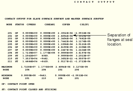
AT NODE 1 1The reaction force is 5.0932 × 10⁻¹¹ N, which is 16 orders of magnitude smaller than the applied load of 200 kN and, thus, is effectively zero. This result confirms that the applied boundary condition, which is not present in the physical problem being simulated, has little effect on the solution.The data file also contains the output from the *CONTACT PRINT option, as shown below for the last increment of the simulation. The parts of the contact surface under the bolted area are closed and sticking. Some shear stress, which developed due to the friction between the surfaces, is transmitted from one surface to the other. The maximum separation of the flanges is 0.28 mm and occurs at the location where the O-ring will be placed.
Examine the results graphically using ABAQUS/Viewer. To begin ABAQUS/Viewer, use the command:
abaqus viewer odb=flangeat the operating system prompt.
Plotting the deformed model shape
You will plot the deformed model shape after assigning different colors to each of the flange components. This will allow you to easily distinguish between the two components.
To change the color of the components:
From the main menu bar, select Tools![]() Color Code.
Color Code.
The Color Code dialog box appears.
Select Element sets from the Method list at the top of the dialog box.
ABAQUS/Viewer displays a default automatic color scheme. The Edge column of the Color mapping table shows asterisks (*) to indicate that the default edge color for the current plot mode will be used. The Color column indicates the colors that ABAQUS/Viewer will use for the element sets.
Click Select All and Deactivate to remove the default color selections.
From the Color Mapping table, select PART-1-1.BOTFLANG and PART-1-1.TOPFLANG.
Edit the color for each element set. Select red as the display color for element set PART-1-1.BOTFLANG and blue as the display color for element set PART-1-1.TOPFLANG.
Click OK to apply the settings and to close the dialog box.
To plot the deformed model shape:
From the main menu bar, select Plot![]() Deformed Shape; or click the
Deformed Shape; or click the ![]() icon in the toolbox to plot the deformed shape.
icon in the toolbox to plot the deformed shape.
Click Deformed Shape Plot Options in the prompt area.
The Deformed Shape Plot Options dialog box appears.
Click Uniform, and enter a uniform deformation scale factor of 10.0.
Set the render style to Shaded.
Click OK to apply the settings and to close the dialog box.
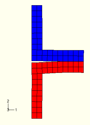
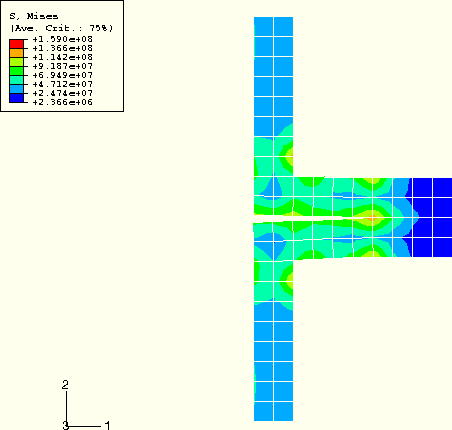
ABAQUS/Viewer displays the deformed model shape at the end of the simulation, as shown in Figure 11–13. Since element faces are now displayed, the edges revert to their default color (black) and the faces reflect the changes made earlier.
From Figure 11–13 we can see the basic results of the analysis. The flanges have been pulled apart at their inner radius, but the bolts have held the outer part of the flanges together. The plot clearly shows the need for an O-ring to help seal this joint.
Reporting values of axial displacement
The separation of the flanges at the seal position can also be determined using ABAQUS/Viewer.
To report the values of displacement:
From the main menu bar, select Tools![]() Query.
Query.
The Query dialog box appears.
From the Visualization Module Queries list, select Probe Values; click OK.
The Probe Values dialog box appears.
Select Nodes, and select Deformed Coordinates in the Probe Values field.
Select the nodes at the seal position: place the cursor over node 2 and click mouse button 1 to save the deformed coordinates. Similarly, select node 202 and save its deformed coordinates.
The deformed coordinates are displayed in the Selected Probe Values field.
The difference between the 2-direction coordinate values is the separation of the flanges at the seal position.
When you have finished querying the nodal displacements and reaction forces, exit from probe mode by clicking Cancel in the Probe Values dialog box. When prompted to write to a file, click No in the dialog box.
Contouring the Mises stress
You will contour the Mises stress in the flanges to assess whether or not the material has yielded.
To contour the Mises stress:
From the main menu bar, select Plot![]() Contours; or click
Contours; or click ![]() in the toolbox to display contours of Mises stress.
in the toolbox to display contours of Mises stress.
Click Contour Options in the prompt area.
The Contour Plot Options dialog box appears.
Drag the Contour Intervals slider bar to change the number of contour intervals to 7.
Click the Shape tab.
The Shape options become available.
Click Uniform, and specify a uniform displacement magnification factor of 10.0.
Click OK to apply the settings and to close the dialog box.
To move the contour legend closer to the model:
From the main menu bar, select Viewport![]() Viewport Annotation Options.
Viewport Annotation Options.
Click the Legend tab in the dialog box that appears.
The Legend options become available.
In the Upper left corner field, set % Viewport X to 15 and % Viewport Y to 90.
Click OK to apply the settings and to close the dialog box.
The legend is moved closer to the model, as shown in Figure 11–14.
The stresses in the two flanges are similar since both are carrying the same load. The peak stress is around 150 MPa. This stress can be compared against the yield stress of the materials to check that the flanges will not yield. It can also be used to determine the fatigue life of the components. However, the mesh used for this analysis is very coarse; it omits geometric details, such as fillet radii, and only includes the effect of the bolts in an approximate manner. Therefore, stress values obtained from this model must be used with caution. A more accurate analysis should be carried out if this preliminary simulation raises any questions about the performance of the flanges.