The interaction between contacting surfaces consists of two components: one normal to the surfaces and one tangential to the surfaces. The tangential component consists of the relative motion (sliding) of the surfaces and, possibly, frictional shear stresses.
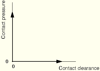
The distance separating two surfaces is called the clearance. The contact constraint is applied when the clearance between two surfaces becomes zero. There is no limit in the contact formulation on the magnitude of contact pressure that can be transmitted between the surfaces. The surfaces separate when the contact pressure between them becomes zero or negative, and the constraint is removed. This surface interaction behavior, referred to as “hard” contact, is summarized in the contact pressure-clearance relationship shown in Figure 11–1.
The dramatic change in contact pressure that occurs when a contact condition changes from “open” (a positive clearance) to “closed” (clearance equal to zero) sometimes makes it difficult to complete contact simulations. Some techniques to overcome difficulties with contact simulations are discussed later in this chapter. Other sources of information include “Common difficulties associated with contact modeling in ABAQUS/Standard,” Section 21.2.9 of the ABAQUS Analysis User's Manual, and the Contact in ABAQUS/Standard lecture notes.In addition to determining whether contact has occurred at a particular point, the analysis also must calculate the relative sliding of the two surfaces. This can be a very complex calculation; therefore, ABAQUS makes a distinction between analyses where the magnitude of sliding is small and those where the magnitude of sliding may be finite. It is much less expensive computationally to model problems where the sliding between the surfaces is small. What constitutes “small sliding” is often difficult to define, but a general guideline to follow is that problems where a point contacting a surface does not slide more than a small fraction of a typical element dimension can use the “small-sliding” approximation.
If the two interacting surfaces are rough, the analysis may need to take frictional forces, which resist the relative sliding of the surfaces, into account. Coulomb friction is a common friction model used to describe the interaction of contacting surfaces. The model characterizes the frictional behavior between the surfaces using a coefficient of friction, ![]() . The product
. The product ![]() , where p is the contact pressure between the two surfaces, gives the limiting frictional shear stress for the contacting surfaces. The contacting surfaces will not slip (slide relative to each other) until the shear stress across their interface equals the limiting frictional shear stress,
, where p is the contact pressure between the two surfaces, gives the limiting frictional shear stress for the contacting surfaces. The contacting surfaces will not slip (slide relative to each other) until the shear stress across their interface equals the limiting frictional shear stress, ![]() . For most surfaces
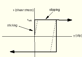
. For most surfaces ![]() is normally less than unity. The solid line in Figure 11–2 summarizes the behavior of the Coulomb friction model: there is zero relative motion (slip) of the surfaces when they are sticking (the shear stresses are below
is normally less than unity. The solid line in Figure 11–2 summarizes the behavior of the Coulomb friction model: there is zero relative motion (slip) of the surfaces when they are sticking (the shear stresses are below ![]() ).
).
The discontinuity between the two states—sticking or slipping—can result in convergence problems during the simulation. You should include friction in your simulations only when it has a significant influence on the response of the model. If your contact simulation with friction encounters convergence problems, one of the first modifications you should try in diagnosing the difficulty is to rerun the analysis without friction.
Simulating the ideal friction behavior can be very difficult; therefore, by default, ABAQUS uses a penalty friction formulation with an allowable “elastic slip,” shown by the dotted line in Figure 11–2. The “elastic slip” is the small amount of relative motion between the surfaces that occurs when the surfaces should be sticking. ABAQUS automatically chooses the penalty stiffness (the slope of the dotted line) so that this allowable “elastic slip” is a very small fraction of the characteristic element length. The penalty friction formulation works well for most problems, including most metal forming applications. In those problems where the ideal stick-slip frictional behavior must be included, the “Lagrange” friction formulation can be used. The “Lagrange” friction formulation is more expensive in terms of the computer resources used because ABAQUS uses additional variables for each surface node with frictional contact. In addition, the solution converges more slowly so that additional iterations are usually required. This friction formulation is not discussed in this guide.
Often the friction coefficient at the initiation of slipping from a sticking condition is different from the friction coefficient during established sliding. The former is typically referred to as the static friction coefficient, and the latter is referred to as the kinetic friction coefficient. In ABAQUS/Standard an exponential decay law is available to model the transition between static and kinetic friction. This friction formulation is not discussed in this guide.
The inclusion of friction in a model adds unsymmetric terms to the system of equations being solved. If ![]() is less than about 0.2, the magnitude and influence of these terms are quite small and the regular, symmetric solver works well (unless the contact surface has high curvature). For higher coefficients of friction, the unsymmetric solver is invoked automatically because it will improve the convergence rate. The unsymmetric solver can also be selected by including the UNSYMM=YES parameter on the *STEP option. The unsymmetric solver requires twice as much computer memory and scratch disk space as the symmetric solver.
is less than about 0.2, the magnitude and influence of these terms are quite small and the regular, symmetric solver works well (unless the contact surface has high curvature). For higher coefficients of friction, the unsymmetric solver is invoked automatically because it will improve the convergence rate. The unsymmetric solver can also be selected by including the UNSYMM=YES parameter on the *STEP option. The unsymmetric solver requires twice as much computer memory and scratch disk space as the symmetric solver.