To demonstrate how to restart an analysis, take the pipe section example in “Example: vibration of a piping system,” Section 10.3, and restart the simulation, adding two additional steps of load history. The first simulation predicted that the piping section would be vulnerable to resonance when extended axially; you must now determine how much additional axial load will increase the pipe's lowest vibrational frequency to an acceptable level.
Step 3 will be a general step that increases the axial load on the pipe to 8 MN, and Step 4 will calculate the eigenmodes and eigenfrequencies again.
Create a new input file, called pipe-2.inp, and add the option blocks discussed below. If you wish to create the entire model using ABAQUS/CAE, refer to “Example: restarting the pipe vibration analysis,” Section 11.5 of Getting Started with ABAQUS.
The only model data required are the *HEADING option and a *RESTART option to read the restart data from the end of the previous analysis. ABAQUS reads all other model data, such as node and element definitions, directly from the restart file. Add the following option blocks to your new input file:
*HEADING
Increase tensile load on the piping system
and determine lowest frequency.
*RESTART, READ
Neither the INCREMENT nor the STEP parameter is included on the *RESTART, READ option since by default ABAQUS will read the data for the last increment written to the restart file. Since you are continuing the simulation from the end of the previous analysis, no parameters are needed.
The history data consist of two steps. Apply a tensile load (8 MN) to the pipe section in Step 3. The following option block must be placed in Step 3:
*CLOAD
RIGHT, 1, 8.0E6
Set the initial time increment in Step 3 to 1/10 the total step time, which should be 1.0. Step 4 is an exact copy of Step 2 from the previous analysis. All of the load history option blocks necessary to define this restart analysis are shown below.
*STEP, NLGEOM
Apply 8 MN axial tensile load
*STATIC
0.1,1.
*CLOAD
RIGHT, 1, 8.0E6
*RESTART, WRITE, FREQUENCY=10
*OUTPUT, FIELD, FREQUENCY=10, VARIABLE=PRESELECT
*OUTPUT, HISTORY
*ELEMENT OUTPUT, ELSET=ELEMENT25
S, SINV
*NODE PRINT, FREQUENCY=0
*EL PRINT, FREQUENCY=0
*END STEP
*STEP, PERTURBATION
Extract modes and frequencies
*FREQUENCY, EIGENSOLVER=SUBSPACE
8,
*RESTART, WRITE
*OUTPUT, FIELD, VARIABLE=PRESELECT
*NODE PRINT, FREQUENCY=0
*EL PRINT, FREQUENCY=0
*END STEP
The complete input file for this restart analysis is listed in “Restarting the pipe vibration analysis,” Section A.11.
When running a simulation that will need to read data from a restart file, you must specify the root name of the restart file, without the .res extension, with the oldjob parameter on the ABAQUS command line. Thus, use the following command to run this restart analysis:
abaqus job=pipe-2 oldjob=pipe
Again, check the status file as the job is running. When the analysis completes, the contents of the status file will look like
 SUMMARY OF JOB INFORMATION:
 STEP  INC ATT SEVERE EQUIL TOTAL  TOTAL      STEP       INC OF       DOF    IF
               DISCON ITERS ITERS  TIME/    TIME/LPF    TIME/LPF    MONITOR RIKS
               ITERS               FREQ
   3     1   1     0     1     1  1.10       0.100      0.1000
   3     2   1     0     1     1  1.20       0.200      0.1000
   3     3   1     0     1     1  1.35       0.350      0.1500
   3     4   1     0     1     1  1.58       0.575      0.2250
   3     5   1     0     1     1  1.91       0.913      0.3375
   3     6   1     0     1     1  2.00       1.00       0.08750
   4     1   1     0     6     0  2.00       1.00e-36   1.000e-36
This analysis starts at Step 3 since Steps 1 and 2 were completed in the previous analysis. There are now two output database (.odb) files associated with this simulation. Data for Steps 1 and 2 are in the file pipe.odb; data for Steps 3 and 4 are in the file pipe-2.odb. When plotting results in ABAQUS/Viewer, you need to remember which results are stored in each file, and you need to ensure that ABAQUS/Viewer is using the correct output database file.
Start ABAQUS/Viewer and specify that the output database file from the restart analysis should be used by giving the following command:
abaqus viewer odb=pipe-2
Plotting the eigenmodes of the pressurized pipe
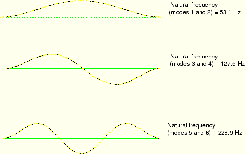
Plot the same six eigenmode shapes of the pipe section for this simulation as were plotted in the previous analysis. The eigenmode shapes can be plotted using the procedures described for the original analysis. These eigenmodes and their natural frequencies are shown in Figure 10–12; again, the corresponding mode shapes lie in planes orthogonal to each other.
Under 8 MN of axial load, the lowest mode is now at 53.1 Hz, which is greater than the required minimum of 50 Hz. If you want to find the exact load at which the lowest mode is just above 50 Hz, you can repeat this restart analysis and change the value of the applied load.
Plotting X–Y graphs for selected steps
Use the results stored in the output database files, pipe.odb and pipe-2.odb, to plot the history of Mises stress in the pipe for the whole simulation.
To generate a history plot of the Mises stress in element 25 for the restart analysis:
From the main menu bar, select Result![]() History Output.
History Output.
The History Output dialog box appears.
Plot the Mises stress history of element 25 at integration point 1 at an angle of 0° with respect to the local 1-axis of the element.
The plot traces the Mises stress history of the element in the restart analysis. Since the restart is a continuation of an earlier job, it is often useful to view the results from the entire (original and restarted) analysis.
To generate a history plot of the Mises stress in element 25 for the entire analysis:
Save the current plot by selecting Result![]() History Output from the main menu. Ensure that the correct quantity has been selected, and click Save As. Name the plot RESTART.
History Output from the main menu. Ensure that the correct quantity has been selected, and click Save As. Name the plot RESTART.
From the main menu bar, select File![]() Open; or use the
Open; or use the ![]() tool in the toolbar to open the file pipe.odb in ABAQUS/Viewer.
tool in the toolbar to open the file pipe.odb in ABAQUS/Viewer.
Following the procedure outlined above, save the plot of the Mises stress history of element 25. Name this plot ORIGINAL.
From the main menu bar, select Tools![]() XY Data
XY Data![]() Manager.
Manager.
The ORIGINAL and RESTART plots are listed in the XY Data Manager dialog box.
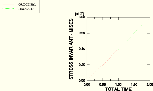
In the XY Data Manager dialog box, select the ORIGINAL and RESTART plots with [Ctrl]+Click, and click Plot to create a plot of Mises stress history of element 25 for the entire simulation.
To change the style of the line, click XY Curve Options in the prompt area.
The XY Curve Options dialog box appears.
For the RESTART curve, select a dotted line style.
Click OK.
To change the plot titles, click XY Plot Options in the prompt area.
The XY Plot Options dialog box appears; by default, the Scale tab is selected. Click the Titles tab.
Click Title source for the X-axis, and select User-specified. Change the title to TOTAL TIME. Similarly, change the Y-axis title to STRESS INVARIANT - MISES.
Click OK.
The plot created by these commands is shown in Figure 10–13.
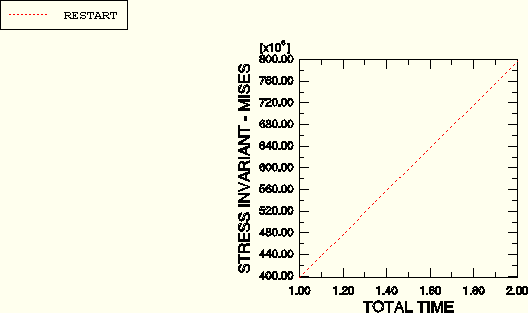
The Mises stress history of the same element during Step 3 can be plotted by itself by selecting only the RESTART curve (see Figure 10–14).