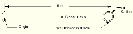
In this example you will study the vibrational frequencies of a 5 m long section of a piping system. The pipe is made of steel and has an outer diameter of 18 cm and a 2 cm wall thickness (see Figure 10–8).
It is clamped firmly at one end and can move only axially at the other end. This 5 m portion of the piping system may be subjected to harmonic loading at frequencies up to 50 Hz. The lowest vibrational mode of the unloaded structure is 40.1 Hz, but this value does not consider how the loading applied to the piping structure may affect its response. To ensure that the section does not resonate, you have been asked to determine the magnitude of the in-service load that is required so that its lowest vibrational mode is higher than 50 Hz. You are told that the section of pipe will be subjected to axial tension when in service. Start by considering a load magnitude of 4 MN.The lowest vibrational mode of the pipe will be a sine wave deformation in any direction transverse to the pipe axis because of the symmetry of the structure's cross-section. You use three-dimensional beam elements to model the pipe section.
The default, global coordinate system is used. Place the origin at the left end of the pipe section, and make the axis of the pipe and the global 1-axis coincident, as shown in Figure 10–8.
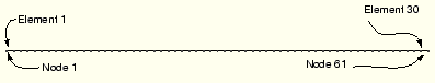
Model the pipe section with a uniformly spaced mesh of 30 second-order, pipe elements (PIPE32). The node and element numbers of the model used in this discussion are shown in Figure 10–9.
You can create the mesh for this example using your preprocessor, or if you prefer, you can use the ABAQUS mesh generation options shown in “Vibration of a piping system,” Section A.10. If you wish to create the entire model using ABAQUS/CAE please refer to “Example: vibration of a piping system,” Section 11.3 of Getting Started with ABAQUS.
The model definition—including the model description, node and element definitions, section properties, and material properties—is discussed next.
Model description
Check that the *HEADING option includes a suitable title in the data lines. Yours should look like the following:
*HEADING
Analysis of a 5 meter long pipe under tensile load
Pipe has OD of 180 mm and ID of 140 mm
S.I. Units
Nodal coordinates and element connectivity
Check that the correct element type (PIPE32) has been used and that the element set names are suitably descriptive.
*ELEMENT, TYPE=PIPE32, ELSET=PIPE
Create node sets containing the nodes at either end of the pipe section. The following option blocks create the node sets for the model shown in Figure 10–9:
*NSET, NSET=LEFT
1
*NSET, NSET=RIGHT
61
Beam properties
The *BEAM SECTION, SECTION=PIPE option will be used with the PIPE32 elements. The outer radius (90 mm) and the wall thickness (20 mm) are needed to define this beam section type geometrically. It is easier to define the orientation of the beam section geometry for this model than it was for the cargo crane model in the earlier chapters because the pipe section is symmetric. Define the approximate ![]() -direction as the vector (0., 0., –1.0). In this model the actual
-direction as the vector (0., 0., –1.0). In this model the actual ![]() -vector will coincide with this approximate vector. The following option block should be in your model:
-vector will coincide with this approximate vector. The following option block should be in your model:
*BEAM SECTION, ELSET=PIPE, MATERIAL=STEEL, SECTION=PIPE
0.09, 0.02
0.0, 0.0, -1.0
Material data
The option blocks defining the material behavior of the steel pipe in your model should look similar to the following:
*MATERIAL, NAME=STEEL
*ELASTIC
200.E9, 0.3
You must define the density of the steel material (7800 kg/m3) because eigenmodes and eigenfrequencies are being extracted in this simulation and a mass matrix is needed for this procedure. Therefore, the following option block must follow the *ELASTIC option block:
*DENSITY
7800.0
In this simulation you need to investigate the eigenmodes and eigenfrequencies of the steel pipe section when a 4 MN tensile load is applied. Therefore, the load history data will be split into two steps:
| Step 1. General step: | Apply a 4 MN tensile force. |
| Step 2. Linear perturbation step: | Calculate modes and frequencies. |
The actual magnitude of time in these steps will have no effect on the results; unless the model includes damping or rate-dependent material properties, “time” has no physical meaning in a static analysis procedure. Therefore, use a step time of 1.0 in the general analysis steps.
Step 1 – Apply a 4 MN tensile force
The options necessary to define the first analysis step—including the procedure definition, boundary conditions, loading, and output requests—are reviewed.
Step and analysis procedure definition
The first step is a general static step that includes the effect of geometric nonlinearity. Specify an initial increment size that is 1/10 the total step time, causing ABAQUS to apply 10% of the load in the first increment. Use the following option blocks to define the analysis procedure, and remember to provide a meaningful description of the step because this makes reviewing the load history much easier:
*STEP, NLGEOM
Apply axial tensile load of 4.0MN
*STATIC
0.1, 1.0
Boundary conditions
The pipe section is clamped at its left end (node 1 in the model shown in Figure 10–9). It is also clamped at the other end; however, the axial force must be applied at this end, so only degrees of freedom 2 to 6 are constrained.
*BOUNDARY
LEFT, 1, 6
RIGHT, 2, 6
Tensile loading
Apply a 4 MN tensile force to the right end of the pipe section such that it deforms in the positive axial (global 1) direction. Forces are applied, by default, in the global coordinate system. Therefore, the *CLOAD option block looks like
*CLOAD
RIGHT, 1, 4.0E6
In this case the load is applied directly to the node set defined earlier. Use the node set name from your model or the node number in the *CLOAD option in your input file.
Output requests
Write data to the restart file every 10 increments. In addition, write the preselected field data every 10 increments as well as the stress components and stress invariants for element 25 as history data to the output database file. Use the FREQUENCY parameter to suppress the node and element printout to the data file. The following option blocks define these output requests:
*ELSET, ELSET=ELEMENT25
25
*RESTART, WRITE, FREQUENCY=10
*OUTPUT, FIELD, FREQUENCY=10, VARIABLE=PRESELECT
*OUTPUT, HISTORY
*ELEMENT OUTPUT, ELSET=ELEMENT25
S, SINV
*NODE PRINT, FREQUENCY=0
*EL PRINT, FREQUENCY=0
End the step with the *END STEP option.
Step 2 – Extract modes and frequencies
The second step extracts the natural frequencies of the extended pipe. The required options are discussed below.
Step and analysis procedure definition
In the second step you need to calculate the eigenmodes and eigenfrequencies of the pipe in its loaded state. The eigenfrequency extraction procedure (*FREQUENCY option) used in this step is a linear perturbation procedure. Although only the first (lowest) eigenmode is of interest to you, extract the first eight eigenmodes for the model. Specify this number on the data line of the *FREQUENCY option block. Since a small number of eigenvalues is requested, use the subspace iteration eigensolver. The option blocks to define the analysis procedure should look similar to the following:
*STEP, PERTURBATION
Extract modes and frequencies
*FREQUENCY, EIGENSOLVER=SUBSPACE
8
Loads
You require the natural frequencies of the extended pipe section. This does not involve the application of any perturbation loads, and the fixed boundary conditions are carried over from the previous general step. Therefore, you do not need to specify any loads or boundary conditions in this step.
Output requests
Any output requests required in a linear perturbation step must be redefined since the requests from the previous general step do not carry over. You want data to be written to the restart and output database files but do not want node or element output to be written to the data file. The following option blocks define these requests:
*RESTART, WRITE
*OUTPUT, FIELD, VARIABLE=PRESELECT
*NODE PRINT, FREQUENCY=0
*EL PRINT, FREQUENCY=0
Again, mark the termination of the step definition with the *END STEP option.
Store the input option blocks in a file called pipe.inp. The input file that creates the model shown in Figure 10–9 is listed in “Vibration of a piping system,” Section A.10. Run the analysis in the background using the command
abaqus job=pipe
Check the status file as the job is running. When the analysis completes, the contents of the status file will look similar to
 SUMMARY OF JOB INFORMATION:
 STEP  INC ATT SEVERE EQUIL TOTAL  TOTAL      STEP       INC OF       DOF    IF
               DISCON ITERS ITERS  TIME/    TIME/LPF    TIME/LPF    MONITOR RIKS
               ITERS               FREQ
   1     1   1     0     1     1  0.100      0.100      0.1000
   1     2   1     0     1     1  0.200      0.200      0.1000
   1     3   1     0     1     1  0.350      0.350      0.1500
   1     4   1     0     1     1  0.575      0.575      0.2250
   1     5   1     0     1     1  0.913      0.913      0.3375
   1     6   1     0     1     1  1.00       1.00       0.08750
   2     1   1     0     4     0  1.00       1.00e-36   1.000e-36
Both steps are shown, and the time associated with the linear perturbation step (Step 2) is very small: the *FREQUENCY procedure, or any linear perturbation procedure, does not contribute to the general loading history of the model.
Run ABAQUS/Viewer using the command
abaqus viewer odb=pipe
Deformed shapes from the linear perturbation steps
When ABAQUS/Viewer starts, it automatically uses the last available frame on the output database file. The results from the second step of this simulation are the natural mode shapes of the pipe and the corresponding natural frequencies. Plot the first mode shape.
To plot the first mode shape:
From the main menu bar, select Result![]() Step/Frame.
Step/Frame.
The Step/Frame dialog box appears.
Select step Extract modes and frequencies and frame Mode 1.
Click OK.
From the main menu bar, select Plot![]() Deformed Shape.
Deformed Shape.
To superimpose the undeformed model shape on the deformed model shape, click Deformed Shape Plot Options in the prompt area.
The Deformed Shape Plot Options dialog box appears.
Toggle on Superimpose undeformed plot.
Click OK.
The undeformed and deformed model shapes are displayed.
To include node symbols for the undeformed shape plot, select Options![]() Undeformed Shape.
Undeformed Shape.
The Undeformed Shape Plot Options dialog box appears; by default, the Basic tab is selected. Click the Labels tab, and toggle on Show node symbols.
It is now possible to select the color, shape, and size of the symbol. Change the color to green and the symbol shape to a solid circle.
Click OK.
Include node symbols for the deformed shape plot using the same procedure described for the undeformed shape plot, selecting Options![]() Deformed Shape from the main menu.
Deformed Shape from the main menu.
The default view is isometric. Try rotating the model to find a better view of the first eigenmode, similar to that shown in Figure 10–10.
Figure 10–10 First and second eigenmode shapes of the pipe section under the tensile load (the modes lie in planes orthogonal to each other).
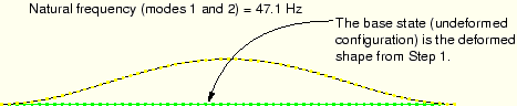
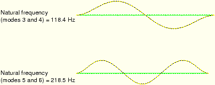
Since this is a linear perturbation step, the undeformed shape is the shape of the structure in the base state. This makes it easy to see the motion relative to the base state. Use the ODB Frame options in the prompt area to plot the other mode shapes. You will discover that this model has many repeated eigenmodes. This is a result of the symmetric nature of the pipe's cross-section, which yields two eigenmodes for each natural frequency, corresponding to the 1–2 and 1–3 planes. The second eigenmode shape is shown in Figure 10–10. Some of the higher vibrational mode shapes are shown in Figure 10–11.
Figure 10–11 Shapes of eigenmodes 3 through 6; corresponding mode shapes lie in planes orthogonal to each other.
The natural frequency associated with each eigenmode will be reported in the plot title. The lowest natural frequency of the pipe section when the 4 MN tensile load is applied is 47.1 Hz. The tensile loading has increased the stiffness of the pipe and, thus, increased the vibrational frequencies of the pipe section. This lowest natural frequency is within the frequency range of the harmonic loads; therefore, resonance of the pipe may be a problem when it is used with this loading.
You, therefore, need to continue the simulation and apply additional tensile load to the pipe section until you find the magnitude that raises the natural frequency of the pipe section to an acceptable level. Rather than repeating the analysis and increasing the applied axial load, you can use the restart capability in ABAQUS to continue the load history of a prior simulation in a new analysis.