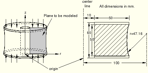
You have been asked to find the axial stiffness of the rubber mount shown in Figure 8–18 and to identify any areas of high maximum principal stress that might limit the fatigue life of the mount. The mount is bonded at both ends to steel plates. It will experience axial loads up to 5.5 kN distributed uniformly across the plates. The cross-section geometry and dimensions are given in Figure 8–18.
You can use axisymmetric elements for this simulation since both the geometry of the model and the loading are axisymmetric. Therefore, you only need to model a plane through the component: each element represents a complete 360° ring.
You do not need to model the whole section of this axisymmetric component because the problem is symmetric about a horizontal line through the center of the mount. By modeling only half of the section, you can use half as many elements and, hence, approximately half the number of degrees of freedom. This significantly reduces the run time and storage requirements for the analysis or, alternatively, allows you to use a more refined mesh.
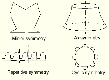
Many problems contain some degree of symmetry. For example, mirror symmetry, cyclic symmetry, axisymmetry, or repetitive symmetry (shown in Figure 8–19) are common. More than one type of symmetry may be present in the structure or component that you want to model.
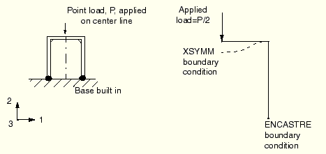
When modeling just a portion of a symmetric component, you have to add boundary conditions to make the model behave as if the whole component were being modeled. You may also have to adjust the applied loads to reflect the portion of the structure actually being modeled. Consider the portal frame in Figure 8–20.
The frame is symmetric about the vertical line shown in the figure. To maintain symmetry in the model, any nodes on the symmetry line must be constrained from translating in the 1-direction and from rotating about the 2- or 3-axes (degrees of freedom 5 and 6). Therefore, the symmetry constraints would be
*BOUNDARY
<node>,1
<node>,5,6
In the frame problem the load is applied along the model's symmetry plane; therefore, only half of the total value should be applied to the portion you are modeling.
In axisymmetric analyses using axisymmetric elements, such as this rubber mount example, we need model only the cross-section of the component. The element formulation automatically includes the effects of axial symmetry.
Use the default r–z (1–2) axisymmetric coordinate system in this simulation. Place the origin at the level of the bottom of the plate, as shown in Figure 8–18.
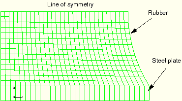
Use a 30 × 15 mesh of first-order, axisymmetric, hybrid solid elements (CAX4H) for the rubber mount. You should include only the bottom half of the mount in your model, as shown in Figure 8–21.
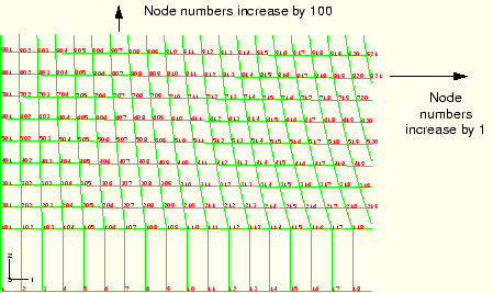
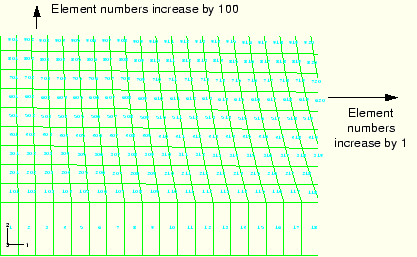
You must use hybrid elements because the material is fully incompressible. The elements are not expected to be subjected to bending, so shear locking in these fully integrated elements should not be a concern. Model the steel plates with a single layer of incompatible mode elements (CAX4I) because it is possible that the plates may bend as the rubber underneath them deforms.The node and element numbers from the input file given in “Axisymmetric mount,” Section A.7, are shown in Figure 8–22 and Figure 8–23. These will be used in the discussion of this example. If you build the model yourself, it will probably have different node and element numbers.
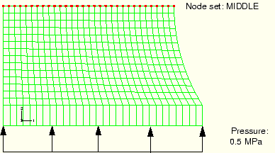
If you use ABAQUS/CAE or another preprocessor to create the mesh for this model, try to create a node set MIDDLE containing all the nodes on the symmetry plane, and apply a pressure load of 0.50 MPa to the bottom of the plate (Figure 8–24). Check that this pressure results in a total applied load of 5.5 kN (5.5 kN = 0.50 MPa × ![]() ). If you can't create the mesh, the ABAQUS input options used to create the model can be found in “Axisymmetric mount,” Section A.7.
). If you can't create the mesh, the ABAQUS input options used to create the model can be found in “Axisymmetric mount,” Section A.7.
If you wish to create the entire model using ABAQUS/CAE, refer to “Example: axisymmetric mount,” Section 10.7 of Getting Started with ABAQUS.
We review the model data, including the geometry definition (nodes and elements) and the material properties.
Model description
Ensure that the input file contains a suitable description of the analysis.
*HEADING
Axisymmetric mount analysis under axial loading.
S.I. Units (m, kg, N, sec)
Nodal coordinates and element connectivity
There will be at least two *ELEMENT option blocks in the input file since two different types of elements are used in the simulation. Check that the element types are correct and that the element sets containing the elements have descriptive names. The *ELEMENT options in your input file should look like
*ELEMENT, TYPE=CAX4I, ELSET=PLATE
*ELEMENT, TYPE=CAX4H, ELSET=RUBBER
Node sets
Check that the node set MIDDLE has been created. If it has not, add it using an editor.
Property definition
Two element property definitions are required: one for the elements modeling the rubber and one for those modeling the plates. The following element property definitions should be in your model:
*SOLID SECTION, MATERIAL=RUBBER, ELSET=RUBBER
*SOLID SECTION, MATERIAL=STEEL, ELSET=PLATE
Material properties: hyperelastic model for the rubber
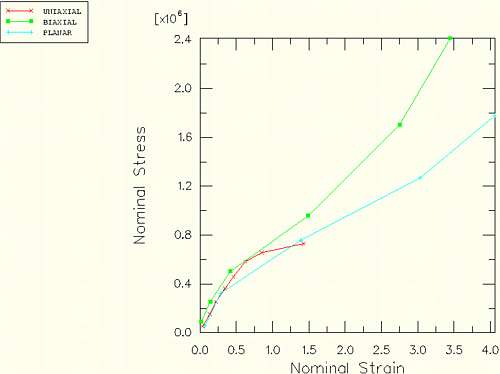
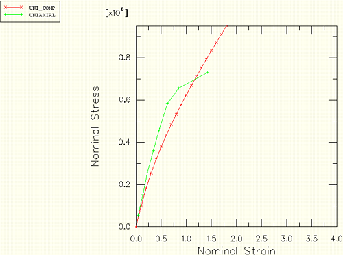
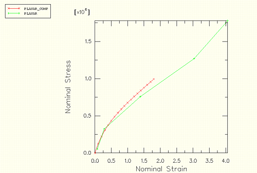
You have been given some experimental test data, shown in Figure 8–25, for the rubber material used in the mount. Three different sets of test data—a uniaxial test, a biaxial test, and a planar (shear) test—are available. You decide to have ABAQUS calculate the appropriate hyperelastic material constants from the test data. You are not sure how large the strains will be in the rubber mount, but you suspect that they will be under 2.0.
The test data for the biaxial and planar tests go well beyond this magnitude, so you decide to perform a one-element simulation of the experimental tests to confirm that the coefficients that ABAQUS calculates from the test data are adequate.Use a first-order, polynomial strain energy function to model the rubber material. Indicate these choices by using the N=1 and POLYNOMIAL parameters on the *HYPERELASTIC option. Use the TEST DATA INPUT parameter to indicate that ABAQUS should find the material constants from the test data you will provide. The test data are given on options that immediately follow the *HYPERELASTIC option. The data should be entered as nominal stress and the corresponding nominal strain, with negative values indicating compression. You may be able to enter the data directly using your preprocessor (for instance, if you are using ABAQUS/CAE); otherwise, you will have to add it to your input file with an editor. The material definition for the rubber will look like
*MATERIAL, NAME=RUBBER
*HYPERELASTIC, N=1, POLYNOMIAL, TEST DATA INPUT
*UNIAXIAL TEST DATA
 0.054E6,  0.0380
 0.152E6,  0.1338
 0.254E6,  0.2210
 0.362E6,  0.3450
 0.459E6,  0.4600
 0.583E6,  0.6242
 0.656E6,  0.8510
 0.730E6,  1.4268
*BIAXIAL TEST DATA
 0.089E6,  0.0200
 0.255E6,  0.1400
 0.503E6,  0.4200
 0.958E6,  1.4900
 1.703E6,  2.7500
 2.413E6,  3.4500
*PLANAR TEST DATA
 0.055E6,  0.0690
 0.324E6,  0.2828
 0.758E6,  1.3862
 1.269E6,  3.0345
 1.779E6,  4.0621
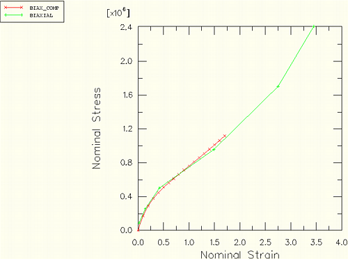
The input file for the single-element simulation of the three experimental tests is shown in “Test fit of hyperelastic material data,” Section A.8. The computational and experimental results for the various types of tests are compared in Figure 8–26, Figure 8–27, and Figure 8–28.
Figure 8–26 Comparison of experimental data (BIAXIAL) and ABAQUS results (BIAX_COMP): biaxial tension.
Material properties: elastic properties for the steel
The steel is modeled with linear elastic properties only (![]() = 200 GPa,
= 200 GPa, ![]() = 0.3) because the loads should not be large enough to cause inelastic deformations. Thus, the material option blocks for the steel are
= 0.3) because the loads should not be large enough to cause inelastic deformations. Thus, the material option blocks for the steel are
*MATERIAL, NAME=STEEL
*ELASTIC
2.0E11,0.3
We now discuss the history data associated with this problem, including the time incrementation parameters, boundary conditions, loading, and output requests.
Including nonlinear geometry and specifying the initial increment size
When hyperelastic materials are used in a model, ABAQUS assumes that it may undergo large deformations. But large deformations and other nonlinear geometric effects are included only if the NLGEOM parameter is used on the *STEP option. Therefore, you must include it in this simulation or ABAQUS will terminate the analysis with an input error. The *STEP option should look like
*STEP, NLGEOM
The simulation will be a static analysis with a total step time of 1.0. Specify the initial time increment to be 1/100th of the total step time. The procedure option block should look like
*STATIC
.01,1.0
Boundary conditions
Specify symmetry boundary conditions on the nodes lying on the symmetry plane. In this model the symmetry conditions prevent the nodes from moving in degree of freedom 2 (axially), as shown in Figure 8–29.
Symmetry conditions that constrain motion in the global 2-direction can be applied using the YSYMM type boundary condition, or you can simply constrain the 2-direction. In this case the *BOUNDARY option block has the following format:*BOUNDARY MIDDLE, 2, 2, 0.0
No boundary constraints are needed in the radial direction (global 1-direction) because the axisymmetric nature of the model does not allow the structure to move as a rigid body in the radial direction. ABAQUS will allow nodes to move in the radial direction, even those initially on the axis of symmetry (i.e., those with a radial coordinate of 0.0), if no boundary conditions are applied to their radial displacements (degree of freedom 1). Since you want to let the mount deform radially in this analysis, do not apply any boundary conditions; again, ABAQUS will prevent rigid body motions automatically.
Loading
The mount must carry a maximum axial load of 5.5 kN, spread uniformly over the steel plates. A distributed load is, therefore, applied to the bottom of the steel plate. The magnitude of the pressure is given by
![]()
If you generated the pressure loading using a preprocessor, a *DLOAD option block with many data lines may be present in the input file.
*DLOAD
 1, P1, 0.50E6
 2, P1, 0.50E6
...
29, P1, 0.50E6
30, P1, 0.50E6
For the element and node numbering discussed here, the pressure is applied to face 1 of all the elements in element set PLATE. This allows us to use a much more compact format for the data lines of the *DLOAD option block.
*DLOAD
PLATE, P1, 0.50E6
Output requests
Use the FREQUENCY parameter to suppress all printed output. Write the preselected variables and nominal strains as field output to the output database file. In addition, write the displacement of one of the nodes on the bottom of the steel plate to the output database file so that the stiffness of the mount can be calculated. You will need to create a node set containing the node. The output option blocks in your model should be similar to the following:
*NODE PRINT, FREQUENCY=0
*EL PRINT, FREQUENCY=0
*NSET, NSET=NODEOUT
1,
*OUTPUT, FIELD, VARIABLE=PRESELECT
*ELEMENT OUTPUT
NE,
*OUTPUT, HISTORY
*NODE OUTPUT, NSET=NODEOUT
U,
Ensure that the end of the step definition is clearly marked with an *END STEP option.
Store your input options in a file called mount.inp. The input options for the model discussed in the above sections can be found in “Axisymmetric mount,” Section A.7. Since the nonlinear nature of the simulation means that it may take some time to complete, use the following command to run the analysis in the background:
abaqus job=mount
When the job has completed, check the data file, mount.dat, for errors. If there are any, correct the input file and rerun the analysis. If necessary, compare your input with that shown in “Axisymmetric mount,” Section A.7.
We briefly review the results associated with the polynomial fit of the test data.
The hyperelastic material parameters
In this simulation you specified that the material is incompressible (![]() =0). The incompressibility is assumed since no volumetric test data were provided. To simulate compressible behavior, you must provide volumetric test data in addition to the other test data. You also specified that ABAQUS should use a first-order, polynomial strain energy function. This form of the hyperelasticity model is known as the Mooney-Rivlin material model.
=0). The incompressibility is assumed since no volumetric test data were provided. To simulate compressible behavior, you must provide volumetric test data in addition to the other test data. You also specified that ABAQUS should use a first-order, polynomial strain energy function. This form of the hyperelasticity model is known as the Mooney-Rivlin material model.
The hyperelastic material coefficients—![]() ,
, ![]() , and
, and ![]() —that ABAQUS calculates from the material test data are given in the data file, mount.dat, provided that you used the *PREPRINT, MODEL=YES option in the model data section of the input file. The material test data are also written in the file so that you can ensure that ABAQUS used the correct data, as shown below.
—that ABAQUS calculates from the material test data are given in the data file, mount.dat, provided that you used the *PREPRINT, MODEL=YES option in the model data section of the input file. The material test data are also written in the file so that you can ensure that ABAQUS used the correct data, as shown below.
                                       M A T E R I A L   D E S C R I P T I O N

  MATERIAL NAME: RUBBER

          UNIAXIAL TEST DATA

          NOMINAL STRESS     NOMINAL STRAIN      TEMP.
             5.4000E+04         3.8000E-02
             1.5200E+05         0.1338
             2.5400E+05         0.2210
             3.6200E+05         0.3450
             4.5900E+05         0.4600
             5.8300E+05         0.6242
             6.5600E+05         0.8510
             7.3000E+05          1.427

          BIAXIAL TEST DATA

          NOMINAL STRESS     NOMINAL STRAIN      TEMP.
             8.9000E+04         2.0000E-02
             2.5500E+05         0.1400
             5.0300E+05         0.4200
             9.5800E+05          1.490
             1.7030E+06          2.750
             2.4130E+06          3.450
          PLANAR TEST DATA

          NOMINAL STRESS     NOMINAL STRAIN      TEMP.
             5.5000E+04         6.9000E-02
             3.2400E+05         0.2828
             7.5800E+05          1.386
             1.2690E+06          3.034
             1.7790E+06          4.062

     HYPERELASTICITY - MOONEY-RIVLIN STRAIN ENERGY

                      D1            C10           C01
                   0.000000E+00   176051.       4332.63
If there were any problems with the stability of the hyperelastic material model, warning messages would be given before the material parameters. The material model is stable at all strains with these material test data and this strain energy function. However, if you specified that a second-order (N=2), polynomial strain energy function be used, you would see the following warnings in the data file:
  *HYPERELASTIC, N=2, POLYNOMIAL, TEST DATA INPUT
***WARNING: UNSTABLE HYPERELASTIC MATERIAL
        FOR UNIAXIAL TENSION WITH A NOMINAL STRAIN LARGER THAN        6.9700
        FOR UNIAXIAL COMPRESSION WITH A NOMINAL STRAIN LESS THAN     -0.9795
        FOR BIAXIAL TENSION WITH A NOMINAL STRAIN LARGER THAN         5.9800
        FOR BIAXIAL COMPRESSION WITH A NOMINAL STRAIN LESS THAN      -0.6458
        FOR PLANE TENSION WITH A NOMINAL STRAIN LARGER THAN           7.0400
        FOR PLANE COMPRESSION WITH A NOMINAL STRAIN LESS THAN        -0.8756

        POLYNOMIAL STRAIN ENERGY FUNCTION WITH N =  2
             D1         C10         C01
             D2         C20         C11         C02
         0.0000E+00  0.1934E+06  -148.2
         0.0000E+00  -805.7       180.0      -3.967
If you only had the uniaxial test data available for this problem, you would find that the Mooney-Rivlin material model ABAQUS creates would have unstable material behavior above certain strain magnitudes.
Use ABAQUS/Viewer to look at the analysis results by issuing the following command:
abaqus viewer odb=mountat the operating system prompt.
Calculating the stiffness of the mount
Determine the stiffness of the mount by creating an X–Y plot of the displacement of the steel plate as a function of the applied load. Create a plot of the vertical displacement of the node on the steel plate for which you wrote data to the output database file. Data were written for node 1 in this model. Swap the X- and Y-axes, and name the plot SWAPPED as shown in the procedure below.
To create a history curve of vertical displacement at node 1 and swap the X- and Y-axes:
From the main menu bar, select Result![]() History Output.
History Output.
The ODB History Output dialog box appears.
In the Output Variables field, use the scroll bar to locate and select the vertical displacement U2 at node 1.
Click Save As to save the X–Y data.
The Save XY Data As dialog box appears.
Type the name DISP, and click OK.
Click Dismiss to close the ODB History Output dialog box.
From the main menu bar, select Tools![]() XY Data
XY Data![]() Create.
Create.
The Create XY Data dialog box appears.
Select Operate on XY data, and click Continue.
The Operate on XY Data dialog box appears.
From the Operators listed, click swap(X).
swap( ) appears in the text field at the top of the dialog box.
In the XY Data field, select DISP and click Add to Expression.
The expression swap( “DISP” ) appears in the text field.
Save the swapped data object by clicking Save As at the bottom of the dialog box.
The Save XY Data As dialog box appears.
In the Name text field, type SWAPPED; and click OK to close the dialog box.
To view the swapped plot of time-displacement, click Plot Expression at the bottom of the dialog box.
You now have a curve of time-displacement. What you need is a curve showing force-displacement. This is easy to create because in this simulation the force applied to the mount is directly proportional to the total time in the analysis. All you have to do to plot a force-displacement curve, called FORCEDEF, is multiply the curve SWAPPED by the magnitude of the load (5.5 kN).
To multiply a curve by a constant value:
In the Operate on XY Data dialog box, click Clear Expression.
In the XY Data field, select SWAPPED and click Add to Expression.
The expression "SWAPPED" appears in the text field at the top of the dialog box.
Click the text field.
The text field becomes highlighted, and the text cursor becomes visible. Place the text cursor at the end of the text field by using either the keyboard arrow buttons or the mouse.
Multiply the data object in the text field by the magnitude of the applied load by entering *5500.
The expression “SWAPPED”*5500 appears in the text field.
Save the multiplied data object by clicking Save As at the bottom of the dialog box.
The Save XY Data As dialog box appears.
In the Name text field, type FORCEDEF; and click OK to close the dialog box.
To view the force-displacement plot, click Plot Expression at the bottom of the dialog box.
You have now created a curve with the force-deflection characteristic of the mount. To get the stiffness, you need to differentiate the curve FORCEDEF. You can do this by using the differentiate( ) operator in the Operate on XY data dialog box.
To obtain the stiffness:
In the Operate on XY Data dialog box, clear the current expression.
From the Operators listed, click differentiate(X).
differentiate( ) appears in the text field at the top of the dialog box.
In the XY Data field, select FORCEDEF and click Add to Expression.
The expression differentiate( "FORCEDEF" ) appears in the text field.
Save the differentiated data object by clicking Save As at the bottom of the dialog box.
The Save XY Data As dialog box appears.
In the Name text field, type STIFF; and click OK to close the dialog box.
To plot the stiffness-displacement curve, click Plot Expression at the bottom of the dialog box.
Click Cancel to close the dialog box.
Click XY Plot Options in the prompt area of the main window.
The XY Plot Options dialog box appears.
Click the Titles tab, and select User-specified as the Title source.
Customize the axis labels as they appear in Figure 8–30 by filling in the Title text fields for the X- and Y-axes.
Click OK to close the XY Plot Options dialog box.
From the main menu bar, select Tools![]() XY Data
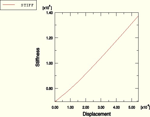
XY Data![]() Plot. From the list of curves select STIFF to view the plot in Figure 8–30 that shows the variation of the mount's axial stiffness as it deforms.
Plot. From the list of curves select STIFF to view the plot in Figure 8–30 that shows the variation of the mount's axial stiffness as it deforms.
To define the stiffness curve directly:
From the main menu bar, select Tools![]() XY Data
XY Data![]() Create.
Create.
The Create XY Data dialog box appears.
Select Operate on XY data, and click Continue.
The Operate on XY Data dialog box appears.
Clear the current expression; and from the Operators listed, click differentiate(X).
differentiate( ) appears in the text field at the top of the dialog box.
From the Operators listed, click swap( X ).
differentiate( swap( ) ) appears in the text field.
In the XY Data field, select DISP and click Add to Expression.
The expression differentiate( swap( “DISP” ) ) appears in the text field.
Place the cursor in the text field directly after the swap( “DISP” ) data object, and type *5500 to multiply the swapped data by the constant total force value.
differentiate( swap( “DISP” )*5500 ) appears in the text field.
Save the differentiated data object by clicking Save As at the bottom of the dialog box.
The Save XY Data As dialog box appears.
In the Name text field, type STIFFNESS; and click OK to close the dialog box.
Click Cancel to close the dialog box.
Click XY Plot Options in the prompt area of the main window.
The XY Plot Options dialog box appears.
Click the Titles tab, and select User-specified as the Title source.
Customize the axis labels as they appear in Figure 8–30 by filling in the Title text fields for the X- and Y- axes.
Click OK to close the XY Plot Options dialog box.
From the main menu bar, select Tools![]() XY Data
XY Data![]() Plot.
Plot.
From the list of curves, select STIFFNESS to view the plot in Figure 8–30 that shows the variation of the mount's axial stiffness as the mount deforms.
Model shape plots
You will now plot the undeformed and deformed model shapes of the mount. The latter plot will allow you to evaluate the quality of the deformed mesh and to assess the need for mesh refinement.
To plot the undeformed and deformed model shapes:
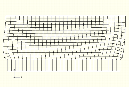
From the main menu bar, select Plot![]() Undeformed Shape; or use the
Undeformed Shape; or use the ![]() tool on the toolbar to plot the undeformed model shape (Figure 8–31).
tool on the toolbar to plot the undeformed model shape (Figure 8–31).
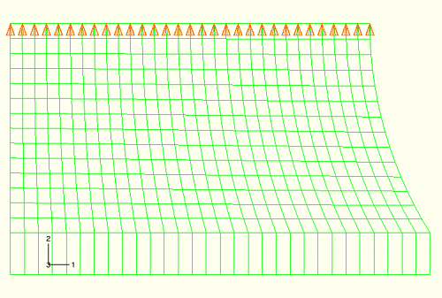
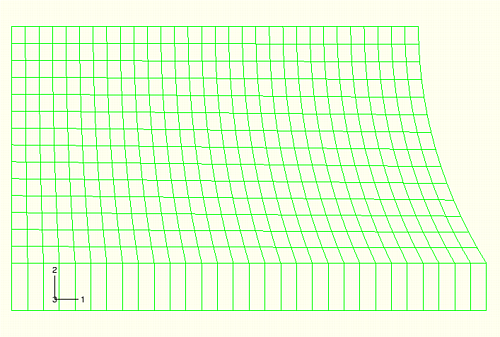
Now plot the deformed model shape (Figure 8–32).
If the figure obscures the plot title, you can move the plot by clicking the ![]() tool and holding down mouse button 1 to pan the deformed shape to the desired location. Alternatively, you can turn the plot title off.
tool and holding down mouse button 1 to pan the deformed shape to the desired location. Alternatively, you can turn the plot title off.
To turn off the title and state blocks:
From the main menu bar, select Viewport![]() Viewport Annotation Options.
Viewport Annotation Options.
The Viewport Annotation Options dialog box appears.
Click the General tab, and toggle off Show title block and Show state block.
Click OK to apply the changes and to close the Viewport Annotation Options dialog box.
The plate has been pushed up, causing the rubber to bulge at the sides.
Zoom in on the bottom left corner of the mesh using the ![]() tool from the toolbar.
tool from the toolbar.
Click mouse button 1, and hold it down to define the first corner of the new view; move the mouse to create a box enclosing the viewing area that you want (Figure 8–33); and release the mouse button. Alternatively, you can zoom and pan the plot by selecting View![]() Specify from the main menu bar.
Specify from the main menu bar.
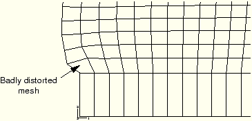
You should have a plot similar to the one shown in Figure 8–33.
Some elements in this corner of the model are becoming badly distorted because the mesh design in this area was inadequate for the type of deformation that occurs there. Although the shape of the elements is fine at the start of the analysis, they become badly distorted as the rubber bulges outward, especially the element in the corner. If the loading were increased further, the element distortion may become so excessive that the analysis may abort. “Mesh design for large distortions,” Section 8.7, discusses how to improve the mesh design for this problem.
The keystoning pattern exhibited by the distorted elements in the bottom right-hand corner of the model indicates that they are locking. A contour plot of the hydrostatic pressure stress in these elements (without averaging across elements sharing common nodes) shows rapid variation in the pressure stress between adjacent elements. (To see this, change the contour type to Quilt in the Contour Plot Options dialog box.) This indicates that these elements are suffering from volumetric locking, which was discussed earlier in “Selecting elements for elastic-plastic problems,” Section 8.3, in the context of plastic incompressibility. Volumetric locking arises in this problem from overconstraint. The steel is very stiff compared to the rubber. Thus, along the bond line the rubber elements cannot deform laterally. Since these elements must also satisfy incompressibility requirements, they are highly constrained and locking occurs. Analysis techniques that address volumetric locking are discussed in “Techniques for reducing volumetric locking,” Section 8.8.
Contouring the maximum principal stress
Plot the maximum in-plane principal stress in the model. Follow the procedure given below to create a filled contour plot on the actual deformed shape of the mount with the plot title suppressed.
To contour the maximum principal stress:
From the main menu bar, select Result![]() Field Output.
Field Output.
The Field Output dialog box appears; by default, the Primary Variable tab is selected.
From the list of output variables, select S.
From the list of invariants, select Max. Principal.
Click OK.
The Select Plot Mode dialog box appears.
Toggle on Contour, and click OK.
ABAQUS/Viewer displays a contour plot of the maximum in-plane principal stresses.You must add the visible edges and set the deformation scale factor to produce the plot shown in Figure 8–34.
Click Contour Options in the prompt area.
The Contour Plot Options dialog box appears.
Drag the uniform contour intervals slider to 8.
Click OK to view the contour plot and to close the dialog box.
Create a display group showing only the elements in the rubber mount.
Select Tools![]() Display Group
Display Group![]() Create.
Create.
The Create Display Group dialog box appears.
From the Item list, select Elements and the PART-1-1.RUBBER element set. Click ![]() to replace the current display group with the PART-1-1.RUBBER element set.
to replace the current display group with the PART-1-1.RUBBER element set.
The viewport display changes and displays only the rubber mount elements.
Click Dismiss to close the Create Display Group dialog box.
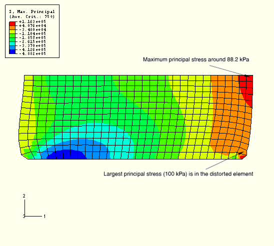
The maximum principal stress in the model, reported in the contour legend, is 135 kPa. Although the mesh in this model is fairly refined and, thus, the extrapolation error should be minimal, you may want to use the query tool ![]() in ABAQUS/Viewer to determine the more accurate integration point values of the maximum principal stress.
in ABAQUS/Viewer to determine the more accurate integration point values of the maximum principal stress.
When you look at the integration point values, you will discover that the peak value of maximum principal stress occurs in one of the distorted elements in the bottom right-hand part of the model. This value is likely to be unreliable because of the levels of element distortion and volumetric locking. If this value is ignored, there is an area near the plane of symmetry where the maximum principal stress is around 88.3 kPa.
The easiest way to check the range of the principal strains in the model is to display the maximum and minimum values in the contour legend.
To check the principal strain magnitude:
From the main menu bar, select Viewport![]() Viewport Annotation Options.
Viewport Annotation Options.
The Viewport Annotation Options dialog box appears.
Click the Legend tab, and toggle on Show min/max values.
Click OK.
The maximum and minimum values appear at the bottom of the contour legend in the viewport.
From the main menu bar, select Result![]() Field Output.
Field Output.
The Field Output dialog box appears; by default, the Primary Variable tab is selected.
From the list of output variables, select NE.
From the list of invariants, select Max. Principal.
Click Apply.
The contour plot changes to display values for maximum principal strain. Note the value of the maximum principal strain from the contour legend.
From the list of invariants in the Field Output dialog box, select Min. Principal.
Click OK to dismiss the Field Output dialog box.
The contour plot changes to display values for minimum principal strain. Note the value of the minimum principal strain from the contour legend.
The maximum and minimum principal nominal strain values indicate that the maximum tensile nominal strain in the model is about 88% and the maximum compressive nominal strain is about 48%. Because the strains in the model remained within the range where the ABAQUS hyperelasticity model has a good fit to the material data, you can be fairly confident that the response predicted by the mount is reasonable from a material modeling viewpoint.