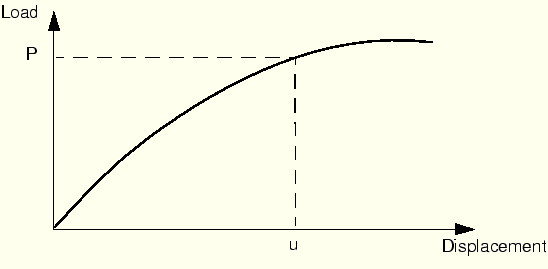
The nonlinear load-displacement curve for a structure is shown in Figure 7–7.
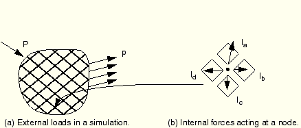
The objective of the analysis is to determine this response. ABAQUS uses the Newton-Raphson method to obtain solutions for nonlinear problems. In a nonlinear analysis the solution cannot be calculated by solving a single system of equations, as would be done in a linear problem. Instead, the solution is found by applying the specified loads gradually and incrementally working toward the final solution. Therefore, ABAQUS breaks the simulation into a number of load increments and finds the approximate equilibrium configuration at the end of each load increment. It often takes ABAQUS several iterations to determine an acceptable solution to a given load increment. The sum of all of the incremental responses is the approximate solution for the nonlinear analysis.Consider the external forces, ![]() , and the internal (nodal) forces,
, and the internal (nodal) forces, ![]() , acting on a body (see Figure 7–8(a) and Figure 7–8(b), respectively). The internal loads acting on a node are caused by the stresses in the elements that contain that node.
, acting on a body (see Figure 7–8(a) and Figure 7–8(b), respectively). The internal loads acting on a node are caused by the stresses in the elements that contain that node.
For the body to be in equilibrium, the net force acting at every node must be zero. Therefore, the basic statement of equilibrium is that the internal forces, ![]() , and the external forces,
, and the external forces, ![]() , must balance each other:
, must balance each other:
![]()
This section introduces some new vocabulary for describing the various parts of an analysis. It is important that you clearly understand the difference between an analysis step, a load increment, and an iteration.
The load history for a simulation consists of one or more steps. You define the steps, which generally consist of an analysis procedure option, loading options, and output request options. Different loads, boundary conditions, analysis procedure options, and output requests can be used in each step. For example:
Step 1: Hold a plate between rigid jaws.
Step 2: Add loads to deform the plate.
Step 3: Find the natural frequencies of the deformed plate.
An increment is part of a step. In nonlinear analyses the total load applied in a step is broken into smaller increments so that the nonlinear solution path can be followed. You suggest the size of the first increment, and ABAQUS automatically chooses the size of the subsequent increments. At the end of each increment the structure is in (approximate) equilibrium and results are available for writing to the output database, restart, data, or results files. The increments at which you select results to be written to the output database file are called frames.
An iteration is an attempt at finding an equilibrium solution in an increment. If the model is not in equilibrium at the end of the iteration, ABAQUS tries another iteration. With every iteration the solution ABAQUS obtains should be closer to equilibrium; sometimes ABAQUS may need many iterations to obtain an equilibrium solution. When an equilibrium solution has been obtained, the increment is complete. Results can be requested only at the end of an increment.
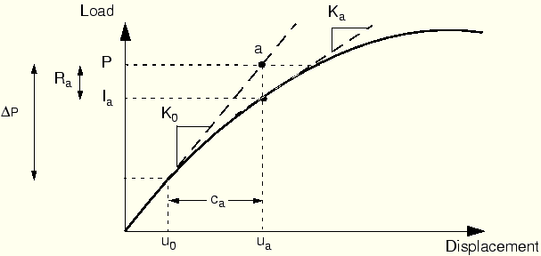
The nonlinear response of a structure to a small load increment, ![]() , is shown in Figure 7–9. ABAQUS uses the structure's initial stiffness,
, is shown in Figure 7–9. ABAQUS uses the structure's initial stiffness, ![]() , which is based on its configuration at
, which is based on its configuration at ![]() , and
, and ![]() to calculate a displacement correction,
to calculate a displacement correction, ![]() , for the structure. Using
, for the structure. Using ![]() , the structure's configuration is updated to
, the structure's configuration is updated to ![]() .
.
Convergence
ABAQUS forms a new stiffness, ![]() , for the structure, based on its updated configuration,
, for the structure, based on its updated configuration, ![]() . ABAQUS also calculates the structure's internal forces,
. ABAQUS also calculates the structure's internal forces, ![]() , in this updated configuration. The difference between the total applied load,
, in this updated configuration. The difference between the total applied load, ![]() , and
, and ![]() can now be calculated as:
can now be calculated as:
![]()
If ![]() is zero at every degree of freedom in the model, point
is zero at every degree of freedom in the model, point ![]() in Figure 7–9 would lie on the load-deflection curve, and the structure would be in equilibrium. In a nonlinear problem it is almost impossible to have
in Figure 7–9 would lie on the load-deflection curve, and the structure would be in equilibrium. In a nonlinear problem it is almost impossible to have ![]() equal zero, so ABAQUS compares it to a tolerance value. If
equal zero, so ABAQUS compares it to a tolerance value. If ![]() is less than this force residual tolerance, ABAQUS accepts the structure's updated configuration as the equilibrium solution. By default, this tolerance value is set to 0.5% of an average force in the structure, averaged over time. ABAQUS automatically calculates this spatially and time-averaged force throughout the simulation.
is less than this force residual tolerance, ABAQUS accepts the structure's updated configuration as the equilibrium solution. By default, this tolerance value is set to 0.5% of an average force in the structure, averaged over time. ABAQUS automatically calculates this spatially and time-averaged force throughout the simulation.
If ![]() is less than the current tolerance value,
is less than the current tolerance value, ![]() and
and ![]() are in equilibrium, and
are in equilibrium, and ![]() is a valid equilibrium configuration for the structure under the applied load. However, before ABAQUS accepts the solution, it also checks that the displacement correction,
is a valid equilibrium configuration for the structure under the applied load. However, before ABAQUS accepts the solution, it also checks that the displacement correction, ![]() , is small relative to the total incremental displacement,
, is small relative to the total incremental displacement, ![]() . If
. If ![]() is greater than 1% of the incremental displacement, ABAQUS performs another iteration. Both convergence checks must be satisfied before a solution is said to have converged for that load increment. The exception to this rule is the case of a linear increment, which is defined as any increment in which the largest force residual is less than 10–8 times the time-averaged force. Any case that passes such a stringent comparison of the largest force residual with the time-averaged force is considered linear and does not require further iteration. The solution is accepted without any check on the size of the displacement correction.
is greater than 1% of the incremental displacement, ABAQUS performs another iteration. Both convergence checks must be satisfied before a solution is said to have converged for that load increment. The exception to this rule is the case of a linear increment, which is defined as any increment in which the largest force residual is less than 10–8 times the time-averaged force. Any case that passes such a stringent comparison of the largest force residual with the time-averaged force is considered linear and does not require further iteration. The solution is accepted without any check on the size of the displacement correction.
If the solution from an iteration is not converged, ABAQUS performs another iteration to try to bring the internal and external forces into balance. This second iteration uses the stiffness, ![]() , calculated at the end of the previous iteration together with
, calculated at the end of the previous iteration together with ![]() to determine another displacement correction,
to determine another displacement correction, ![]() , that brings the system closer to equilibrium (point
, that brings the system closer to equilibrium (point ![]() in Figure 7–10).
in Figure 7–10).
ABAQUS calculates a new force residual, ![]() , using the internal forces from the structure's new configuration,
, using the internal forces from the structure's new configuration, ![]() . Again, the largest force residual at any degree of freedom,
. Again, the largest force residual at any degree of freedom, ![]() , is compared against the force residual tolerance, and the displacement correction for the second iteration,
, is compared against the force residual tolerance, and the displacement correction for the second iteration, ![]() , is compared to the increment of displacement,
, is compared to the increment of displacement, ![]() . If necessary ABAQUS performs further iterations.
. If necessary ABAQUS performs further iterations.
For each iteration in a nonlinear analysis ABAQUS forms the model's stiffness matrix and solves a system of equations. This means that each iteration is equivalent, in computational cost, to conducting a complete linear analysis. It should now be clear that the computational expense of a nonlinear analysis can be many times greater than for a linear one.
It is possible with ABAQUS to save results at each converged increment. Thus, the amount of output data available from a nonlinear simulation is many times that available from a linear analysis of the same geometry. Consider both of these factors and the types of nonlinear simulations that you want to perform when planning your computer resources.
ABAQUS automatically adjusts the size of the load increments so that it solves nonlinear problems easily and efficiently. You only need to suggest the size of the first increment in each step of your simulation. Thereafter, ABAQUS automatically adjusts the size of the increments. If you do not provide a suggested initial increment size, ABAQUS will try to apply all of the loads defined in the step in the first increment. In highly nonlinear problems ABAQUS will have to reduce the increment size repeatedly, resulting in wasted CPU time. Generally it is to your advantage to provide a reasonable initial increment size (see “Modifications to the input filethe history data,” Section 7.4.1, for an example); only in very mildly nonlinear problems can all of the loads in a step be applied in a single increment.
The number of iterations needed to find a converged solution for a load increment will vary depending on the degree of nonlinearity in the system. By default, if the solution has not converged within 16 iterations or if the solution appears to diverge, ABAQUS abandons the increment and starts again with the increment size set to 25% of its previous value. An attempt is then made at finding a converged solution with this smaller load increment. If the increment still fails to converge, ABAQUS reduces the increment size again. By default, ABAQUS allows a maximum of five cutbacks of increment size in an increment before stopping the analysis.
If the increment converges in fewer than five iterations, this indicates that the solution is being found fairly easily. Therefore, ABAQUS automatically increases the increment size by 50% if two consecutive increments require fewer than five iterations to obtain a converged solution.
Details of the automatic load incrementation scheme are given in the message file, as shown in more detail in “Results,” Section 7.4.3.