You have been asked to model the plate shown in Figure 5–10. It is skewed 30° to the global 1-axis, is built-in at one end, and is constrained to move on rails parallel to the plate axis at the other end. You are to determine the midspan deflection when the plate carries a uniform pressure. You are also to assess whether a linear analysis is valid for this problem.
The orientation of the structure in the global coordinate system and the suggested origin of the system are shown in Figure 5–10. The plate lies in the global 1–2 plane. Will it be easy to interpret the results of the simulation if you use the default material directions for the shell elements in this model?
Figure 5–11 shows the suggested mesh for this simulation. The node and element numbers shown were created by the input file in “Skew plate,” Section A.3. The numbering in your model will almost certainly be different.
You must answer the following questions before selecting an element type: Is the plate thin or thick? Are the strains small or large? The plate is quite thin, with a thickness-to-minimum span ratio of 0.02. (The thickness is 0.8 cm and the minimum span is 40 cm.) While we cannot readily predict the magnitude of the strains in the structure, we think that the strains will be small. Based on this information, you choose quadratic shell elements (S8R5), because they give accurate results for thin shells in small-strain simulations. For further details on shell element selection, consult “Choosing a shell element,” Section 15.6.2 of the ABAQUS Analysis User's Manual.
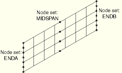
Use a preprocessor such as ABAQUS/CAE to generate the mesh shown in Figure 5–11. Create the node sets shown in Figure 5–12, and put all of the elements in an element set called PLATE.
You can define most of this model in your preprocessor, but leave out the material and history information so you can add it later with an editor. This exercise will give you a better understanding of how the various option blocks combine to define an ABAQUS model. If you do not have a preprocessor, use the ABAQUS mesh generation options described in “Skew plate,” Section A.3. If you wish to create the entire model using ABAQUS/CAE, refer to “Example: skew plate,” Section 5.5 of Getting Started with ABAQUS.Before you start to build the model, decide on a system of units. The dimensions are given in cm, but the loading and material properties are given in MPa and GPa. Since these are not consistent units, you must choose a consistent system to use in your model and convert the necessary input data.
At this point we assume that you have created the basic mesh using your preprocessor. In this section you will review and make corrections to your input file, as well as include additional information, such as material data.
Model description
The following would be a suitable description in the *HEADING option for this simulation:
*HEADING
Linear Elastic Skew Plate. 20 kPa Load.
S.I. Units (meters, Newtons, sec, kilograms)
It clearly explains what you are modeling and what units you are using.
Element connectivity
Check to make sure that you are using the correct element type (S8R5). It is possible that you specified the wrong element type in the preprocessor or that the translator made a mistake when generating the input file. The *ELEMENT option block in your model should begin with the following:
*ELEMENT, TYPE=S8R5, ELSET=PLATEThe name given for the ELSET parameter in your model may not be PLATE. If necessary, change the value to PLATE. Meaningful names for node and element sets make input files easy to understand.
Node sets
The three node sets shown in Figure 5–12 will be useful in completing the model of the plate. If you were unable to define them with your preprocessor, use a text editor and the *NSET option to create node sets with these names.
Defining alternative material directions
If you use the default material directions, the direct stress in the material 1-direction, ![]() , will contain contributions from both the axial stress, produced by the bending of the plate, and the stress transverse to the axis of the plate. It will be easier to interpret the results if the material directions are aligned with the axis of the plate and the transverse direction. Therefore, a local rectangular coordinate system is needed in which the local
, will contain contributions from both the axial stress, produced by the bending of the plate, and the stress transverse to the axis of the plate. It will be easier to interpret the results if the material directions are aligned with the axis of the plate and the transverse direction. Therefore, a local rectangular coordinate system is needed in which the local ![]() -direction lies along the axis of the plate (i.e., at 30° to the global 1-axis) and the local
-direction lies along the axis of the plate (i.e., at 30° to the global 1-axis) and the local ![]() -direction is also in the plane of the plate.
-direction is also in the plane of the plate.
As you learned in “Shell material directions,” Section 5.3, the *ORIENTATION option defines such a local coordinate system. Choose point ![]() (see Figure 5–8) to have coordinates (10.0E–2, 5.77E–2, 0.)—so that
(see Figure 5–8) to have coordinates (10.0E–2, 5.77E–2, 0.)—so that ![]() = tan 30°—and point b to have coordinates (–5.77E–2, 10.E–2, 0.). You must also specify which axis is not projected onto the shell surface (the
= tan 30°—and point b to have coordinates (–5.77E–2, 10.E–2, 0.). You must also specify which axis is not projected onto the shell surface (the ![]() -direction in this model) as well as an additional rotation (zero using this method). Use the following *ORIENTATION option block to create the proper local coordinate system, named SKEW:
-direction in this model) as well as an additional rotation (zero using this method). Use the following *ORIENTATION option block to create the proper local coordinate system, named SKEW:
*ORIENTATION, NAME=SKEW, SYSTEM=RECTANGULAR
10.0E-2,5.77E-2,0.0, -5.77E-2,10.0E-2,0.0
3, 0.0
Alternatively, you can define exactly the same local coordinate system by choosing point
*ORIENTATION, NAME=SKEW, SYSTEM=RECTANGULAR
1., 0., 0., 0., 1., 0.
3, 30.
Section properties
Since the structure is made of a single material with constant thickness, the section properties are the same for all elements. Therefore, you can use the element set PLATE (which includes all elements) to assign the physical and material properties to the elements. Since you assume that the plate is linear elastic, the *SHELL GENERAL SECTION option is more efficient than using the *SHELL SECTION option. Use the following element property option block in your model:
*SHELL GENERAL SECTION, ELSET=PLATE, MATERIAL=MAT1,
ORIENTATION=SKEW
0.8E-2,
The ORIENTATION parameter tells ABAQUS to use the local coordinate system named SKEW to define the material directions for the shells in element set PLATE. All element variables will be defined in the SKEW coordinate system.
Material properties
The plate is made of an isotropic, linear elastic material that has a Young's modulus of 30.0 GPa and a Poisson's ratio of 0.3. Use the following material option block in your model:
*MATERIAL, NAME=MAT1
*ELASTIC
30.0E9, 0.3
Local directions at the nodes
While the *ORIENTATION option defines a local coordinate system for elements, you must use the *TRANSFORM option to define a local coordinate system for nodes. The two options are completely independent of each other. If a node refers to a local coordinate system defined with *TRANSFORM, all data pertaining to the node—such as boundary conditions, concentrated loads, or nodal output variables (displacements, velocities, reaction forces, etc.)—are defined in the transformed coordinate system.
The *TRANSFORM option has the following format:
*TRANSFORM, NSET=<node set name>, TYPE=<axis type> <The data line specifies the coordinates of two points,>, <
>, <
>, <
>, <
>, <
>
As shown in Figure 5–10, one end of the plate is constrained to move on rails that are parallel to the axis of the plate. Since this boundary condition does not coincide with the global axes, you must transform the nodes on this end of the plate into a local coordinate system that has an axis aligned with the plate. Use the following *TRANSFORM option:
*TRANSFORM, NSET=ENDB, TYPE=R
10.0E-2,5.77E-2,0.0, -5.77E-2,10.0E-2,0.0
This option block defines the degrees of freedom for node set ENDB in a local coordinate system whose
We now review the history definition portion of the input file. A single step is needed to define this simulation.
Step definition
Your choice of *STEP definition must reflect the fact that this is a linear, static simulation. If the preprocessor did not create the option blocks to define the step, add the following:
*STEP, PERTURBATION
Uniform pressure (20.0 kPa) load
*STATIC
The line following *STEP, PERTURBATION contains a clear description of the loading applied in this step.
Boundary conditions
The nodes at the left-hand end of the plate (node set ENDA) need to be constrained completely. If necessary, add the following to your input file:
*BOUNDARY
ENDA, ENCASTRE
The nodes at the right-hand end of the plate need to be constrained to model their “rail” boundary condition. Since you have transformed the nodes at this end using *TRANSFORM, you must apply the boundary conditions in the local coordinate system. To allow these nodes to move in the local 1-direction (along the axis of the plate) only, all other degrees of freedom must be constrained as follows:
ENDB, 2,6Had you not defined node sets ENDA and ENDB, you would have had to create a data line for each node.
Loading
A distributed pressure load of 20.0 kPa is applied to the plate in this simulation. As shown in Figure 5–10, the pressure acts in the negative global 3-direction. Pressure loads are applied to the faces of elements with the *DLOAD option (*DLOAD is described in Chapter 4, “Using Continuum Elements,” for the lug model example). Shell elements have only one face; therefore, the load identifier for pressure is just “P.” A positive pressure on a shell acts in the direction of the positive element normal. The shell elements in the input file from “Skew plate,” Section A.3, have normals that align with the positive global 3-axis. Thus, the following input defines the correct pressure loading in that model:
*DLOAD
PLATE, P, -20000.0
Since element set PLATE contains all elements in the model, this option block applies a pressure load to all elements in the model.
Output requests
If the preprocessor has generated default output request options, you should delete them. To create an output database ( .odb) file for use with ABAQUS/Viewer and printed tables of the element stresses, nodal reaction forces, and displacements at the midspan of the plate, add the following output requests to your input file:
*OUTPUT, FIELD, OP=NEW
*NODE OUTPUT
U,
*ELEMENT OUTPUT
S,
*OUTPUT, HISTORY, OP=NEW
*NODE OUTPUT, NSET=MIDSPAN
U,
*EL PRINT
S,
*NODE PRINT, SUMMARY=NO, TOTALS=YES, GLOBAL=YES
RF,
*NODE PRINT, NSET=MIDSPAN
U,
Specifying the *OUTPUT option overrides the default output selections noted in the previous chapters. The option is used with the FIELD and HISTORY parameters to request field and history output to the output database file. In general, field output is used to generate contour plots, symbol plots, and deformed shape plots; history output is used for X–Y plotting. In conjunction with the *OUTPUT option, the *NODE OUTPUT option is used to request output of nodal variables and the *ELEMENT OUTPUT option is used for output of element variables.
You may also want output to be written to a results file, skew.fil, for use with a third-party postprocessor. Use the *NODE FILE and *EL FILE options, which are very similar in format to the *NODE PRINT and *EL PRINT options, to specify which results are to be stored in the results file. The following input stores the displacements at all nodes and the stresses in all elements in the results file:
*NODE FILE
U,
*EL FILE
S,
*END STEP
After storing your input in a file called skew.inp, run the analysis interactively. If you do not remember how to run the analysis, see “Running the analysis,” Section 4.3.6. If your analysis does not complete, check the data file, skew.dat, for error messages. Modify your input file to remove the errors; if you still have trouble running your model, compare your input file to the one given in “Skew plate,” Section A.3.
After running the simulation successfully, look at the table of stresses in the data file, skew.dat. An excerpt from the table is shown below.

Check that the small-strain assumption was valid for this simulation. The axial strain corresponding to the peak stress is ![]() 0.0066. Since the strain is typically considered small if it is less than 4 or 5%, a strain of 0.0066 is well within the appropriate range to be modeled with S8R5 elements.
0.0066. Since the strain is typically considered small if it is less than 4 or 5%, a strain of 0.0066 is well within the appropriate range to be modeled with S8R5 elements.
Look at the reaction forces and moments in the following table:
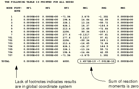
The table of displacements (which is not shown here) shows that the mid-span deflection across the plate is 5.3 cm, which is approximately 5% of the plate's length. By running this as a linear analysis, we assume the displacements to be small. It is questionable whether these displacements are truly small relative to the dimensions of the structure; nonlinear effects may be important, requiring further investigation. In this case we need to perform a geometrically nonlinear analysis, which is discussed in Chapter 7, “Nonlinearity.”
While you have been able to answer this simulation's important questions using the printed output in the data file, more complicated simulations often require graphical postprocessing. This section discusses postprocessing with ABAQUS/Viewer. Both contour and symbol plots are useful for visualizing shell analysis results. Since contour plotting was discussed in detail in Chapter 4, “Using Continuum Elements,” we use symbol plots here.
Start ABAQUS/Viewer by typing
abaqus viewer odb=skewat the operating system prompt.
By default, ABAQUS/Viewer plots the fast representation of the model. Plot the undeformed model shape by selecting Plot![]() Undeformed Shape from the main menu bar or by clicking the
Undeformed Shape from the main menu bar or by clicking the ![]() tool in the toolbox.
tool in the toolbox.
Element normals
Use the undeformed shape plot to check the model definition. Check that the element normals for the skew-plate model were defined correctly and point in the positive 3-direction.
To display the element normals:
In the prompt area, click Undeformed Shape Plot Options.
The Undeformed Shape Plot Options dialog box appears.
Set the render style to Shaded.
Click the Normals tab.
Toggle on Show Normals, and accept the default setting of On elements.
Click OK to apply the settings and to close the dialog box.
The default view is isometric. You can change the view using the options in the view menu or the view tools (such as ![]() ) from the toolbar.
) from the toolbar.
To change the view:
From the main menu bar, select View![]() Specify.
Specify.
The Specify View dialog box appears.
From the list of available methods, select Viewpoint.
Enter the ![]() -,
-, ![]() - and
- and ![]() -coordinates of the viewpoint vector as –0.2, –1, 0.8 and the coordinates of the up vector as 0, 0, 1.
-coordinates of the viewpoint vector as –0.2, –1, 0.8 and the coordinates of the up vector as 0, 0, 1.
Click OK.
ABAQUS/Viewer displays your model in the specified view, as shown in Figure 5–13.
Symbol plots
Symbol plots display the specified variable as a vector originating from the node or element integration points. You can produce symbol plots of most tensor- and vector-valued variables. The exceptions are mainly non-mechanical output variables and element results stored at nodes, such as nodal forces. The relative size of the arrows indicate the relative magnitude of the results, and the vectors are oriented along the global direction of the results. You can plot results for the resultant of variables such as displacement (U), reaction force (RF), etc., or you can plot individual components of these variables.
To generate a symbol plot of the displacement:
From the main menu bar, select Result![]() Field Output.
Field Output.
The Field Output dialog box appears; by default, the Primary Variable tab is selected.
From the list of output variables, select U.
From the list of components, select U3.
Click OK.
The Select Plot Mode dialog box appears.
Toggle on Symbol, and click OK.
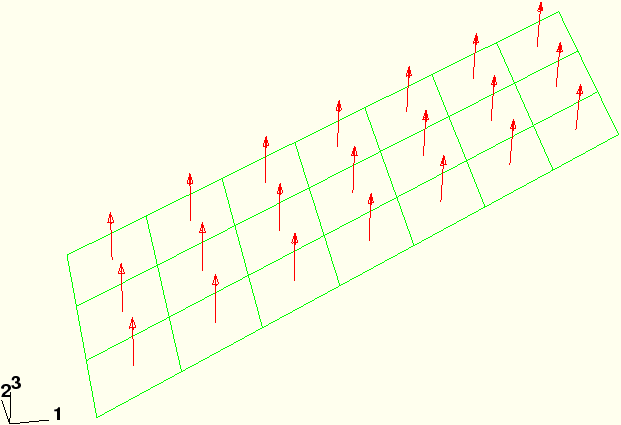
ABAQUS/Viewer displays a symbol plot of the displacements in the 3-direction on the deformed model shape.
To modify the attributes of the symbol plot, click Symbol Options in the prompt area.
The Symbol Plot Options dialog box appears; by default, the Basic tab is selected.
To plot the symbols on the undeformed model shape, click the Shape tab and toggle on Undeformed shape.
Click OK to apply the settings and to close the dialog box.
A symbol plot on the undeformed model shape appears, as shown in Figure 5–14.
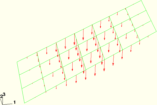
You can plot principal values of tensor variables such as stress using symbol plots. A symbol plot of the principal values of stress yields three vectors at every integration point, each corresponding to a principal value oriented along the corresponding principal direction. Compressive values are indicated by arrows pointing toward the integration point, and tensile values are indicated by arrows pointing away from the integration point. You can also plot individual principal values.
To generate a symbol plot of the principal stresses:
From the main menu bar, select Result![]() Field Output.
Field Output.
The Field Output dialog box appears.
From the list of output variables, select S; and from the list of invariants, select Max. Principal.
Click OK to apply the settings and to close the dialog box.
ABAQUS/Viewer displays a symbol plot of principal stresses.
To change the arrow length, click Symbol Options in the prompt area.
The Symbol Plot Options dialog box appears.
Click the Color & Style tab; then click the Tensor tab.
Drag the Size slider to select 2 as the arrow length.
Click OK to apply the settings and to close the dialog box.
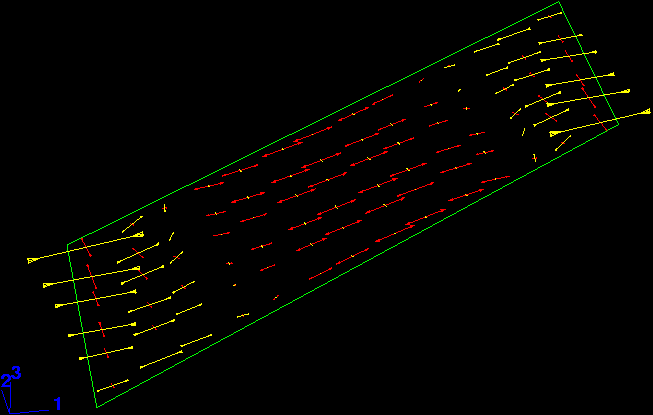
The symbol plot shown in Figure 5–15 appears.
The principal stresses are displayed at section point 1 by default. To plot stresses at non-default section points, select Result![]() Section Points from the main menu bar to bring up the Section Points dialog box.
Section Points from the main menu bar to bring up the Section Points dialog box.
Select the desired non-default section point for plotting.
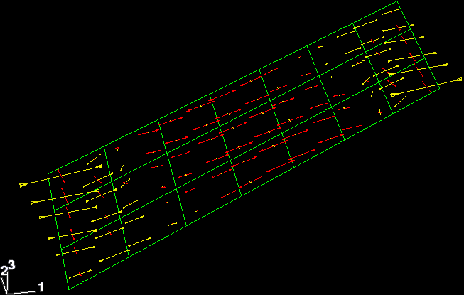
In a complex model, the element edges can obscure the symbol plots. To suppress the display of the element edges, choose Feature visible edges on the Basic page in the Symbol Plot Options dialog box. Figure 5–16 shows a symbol plot of the principal stresses with only feature edges visible.
Material directions
ABAQUS/Viewer also lets you visualize the element material directions. This feature is particularly helpful, allowing you to ensure the correctness of the material directions.
To plot the material directions:
From the main menu bar, select Plot![]() Material Orientations; or click the
Material Orientations; or click the ![]() tool in the toolbox.
tool in the toolbox.
The material orientation directions are plotted on the deformed shape. By default, the triads that represent the material orientation directions are plotted without arrowheads.
To display the triads with arrowheads, click Material Orientation Options in the prompt area.
The Material Orientation Plot Options dialog box appears.
Click the Color & Style tab; then click the Triad tab.
Set the Arrowhead option to use filled arrowheads in the triad.
Click OK to apply the settings and to close the dialog box.
From the main menu bar, select View![]() Views Toolbox; or click the
Views Toolbox; or click the ![]() tool in the toolbar.
tool in the toolbar.
The Views toolbox appears.
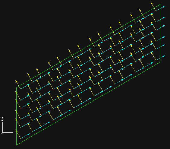
Use the predefined views available in the toolbox to display the plate as shown in Figure 5–17. In this figure, perspective is turned off. To turn off perspective, click the ![]() tool in the toolbar.
tool in the toolbar.
By default, the material 1-direction is colored blue, the material 2-direction is colored yellow, and, if it is present, the material 3-direction is colored red.