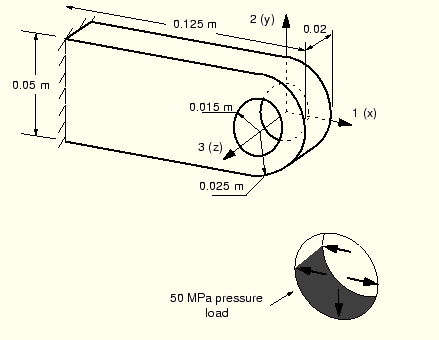
In this example you will use three-dimensional, continuum elements to model the connecting lug shown in Figure 4–14.
The lug is welded firmly to a massive structure at one end. The other end contains a hole. When it is in service, a bolt will be placed through the hole of the lug. You have been asked to determine the deflection of the lug when a 30 kN load is applied to the bolt in the negative 2-direction. You decide to simplify this problem by making the following assumptions:
Rather than include the complex bolt-lug interaction in the model, you will use a distributed pressure over the bottom half of the hole to load the connecting lug (see Figure 4–14).
You will neglect the variation of pressure magnitude around the circumference of the hole and use a uniform pressure.
The magnitude of the applied uniform pressure will be 50 MPa (30 kN/ 2 × 0.015 m × 0.02 m).
In your model define the global 1-axis to lie along the length of the lug, the global 2-axis to be vertical, and the global 3-axis to lie in the thickness direction. Place the origin of the global coordinate system ( ![]() ) at the center of the hole on the
) at the center of the hole on the ![]() face (see Figure 4–14).
face (see Figure 4–14).
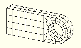
You need to consider the type of element that will be used before you start building the mesh for a particular problem. A suitable mesh design that uses quadratic elements may very well be unsuitable if you change to linear, reduced-integration elements. For this example use 20-node hexahedral elements with reduced integration (C3D20R). With the element type selected, you can design the mesh for the connecting lug. The most important decision regarding the mesh design for this application is how many elements to use around the circumference of the lug's hole. A possible mesh for the connecting lug is shown in Figure 4–15; you should build your model to be similar to it.
Another thing to consider when designing a mesh is what type of results you want from the simulation. The mesh in Figure 4–15 is rather coarse and, therefore, unlikely to yield accurate stresses. Four quadratic elements per 90° is the minimum number that should be considered for a problem like this one; using twice that many is recommended to obtain reasonably accurate stress results. However, this mesh should be adequate to predict the overall level of deformation in the lug under the applied loads, which is what you were asked to determine. The influence of increasing the mesh density used in this simulation is discussed in “Mesh convergence,” Section 4.4.
You need to decide what system of units to use in your model. The SI system of meters, seconds, and kilograms is recommended, but use another system if you prefer.
The model for the overhead hoist in Chapter 2, “ABAQUS Basics,” was simple enough that the ABAQUS input file could be created by typing the input directly into a text editor. This clearly is impractical for most real problems; the input for the examples in this guide can be created easily using ABAQUS/CAE or another preprocessor.
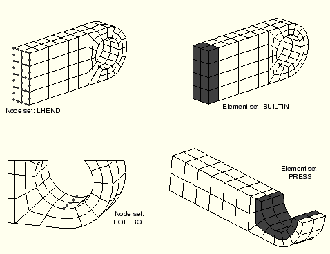
Use a preprocessor to generate the mesh, the node and element sets shown in Figure 4–16, and the pressure load and boundary conditions shown in Figure 4–14. The following discussion assumes that you have done this. Although most preprocessors can create the entire input file for this simulation, it is suggested that you generate only the mesh, the element and node sets shown, and the correct pressure loads and boundary conditions using the preprocessor. You should then add the additional data needed for the model with an editor to obtain a better understanding of the format of an ABAQUS input file. If you do not have a preprocessor, use the ABAQUS mesh generation options in “Connecting lug,” Section A.2. If you wish to create the entire model using ABAQUS/CAE, refer to “Example: connecting lug,” Section 4.3 of Getting Started with ABAQUS.
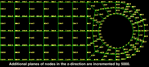
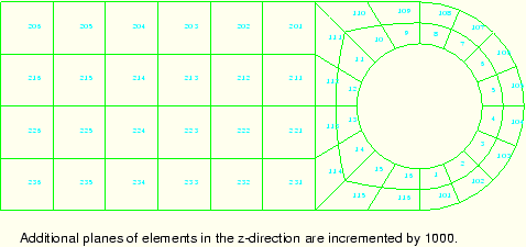
In the description of this simulation that follows, the node and element numbers used are from the model found in “Connecting lug,” Section A.2. These node and element numbers are shown in Figure 4–17 and Figure 4–18. If you use a preprocessor, the node and element numbering in your model will almost certainly differ from that shown here. As you make modifications to your input file, remember to use the node and element numbers in your model and not those given here.
The model data—including the node and element definitions, set definitions, and section and material properties—are discussed in the following sections.
Model description
An ABAQUS input file always starts with the *HEADING option. Often the description given in this option by the preprocessor is not very informative, although it might give the date and time when the file was generated. You should provide a suitable title on the data lines of this option so that someone looking at this file can tell what is being modeled and what units you used. You should modify the *HEADING option block in your file to look like the following:
*HEADING
Linear Elastic Steel Connecting Lug
S.I. Units (N, kg, m, s)
Nodal coordinates and element connectivity
In input files created by a preprocessor, the model's nodal coordinates usually are in one large *NODE option block, with the coordinates specified for each node individually.
The element definitions generated by the preprocessor usually are contained in several *ELEMENT option blocks. Typically, each block contains elements that have the same element section and material properties. In the connecting lug model only one element type is used, and all the elements have the same properties. Therefore, there will probably be a single *ELEMENT option block in your input file. It will look similar to
*ELEMENT, TYPE=C3D20R, ELSET=LUG
   1,     1,   401,   405,     5, 10001, 10401, 10405, 10005,
 201,   403,   205,     3, 10201, 10403, 10205, 10003,
5001,  5401,  5405,  5005
2,        5,   405,   409,     9,  10005, 10405, 10409, 10009,
205,    407,   209,     7, 10205, 10407, 10209, 10007,
5005,  5405,  5409,  5009
.......
It takes three data lines to define the connectivity of one C3D20R element completely. If a data line in an *ELEMENT option block ends with a comma, it indicates that the next data line contains more nodes defining the current element. The parameter ELSET=LUG indicates that all the elements defined in the following data lines will be stored in an element set called LUG. If your model does not have a descriptive element set name in the *ELEMENT option, change it to LUG.
Node and element sets
The node and element sets are important components of an ABAQUS input file because they allow you to assign loads, boundary conditions, and material properties efficiently. They also offer great flexibility in defining the output that your simulation will produce and make it much easier to understand the input file.
Some preprocessors, such as ABAQUS/CAE, will allow you to select and name groups of entities, such as nodes and elements, as you build the model; when the ABAQUS input file is created, node and element sets are generated from these groups.
You define sets using the *NSET and *ELSET options in the input file. The name of a set is specified with either the NSET or ELSET parameter. The data lines list the nodes or elements that are included in the set. Each data line can contain up to 16 numbers, and there can be as many data lines as required. For example, the node set LHEND (see Figure 4–16) can be defined as
*NSET, NSET=LHEND
 3241,  3243,  3245,  3247,  3249,  3251,  3253,  3255, 3257,
 8241,  8245,  8249,  8253,  8257, 13241, 13243, 13245, 13247,
13249, 13251, 13253, 13255, 13257, 18241, 18245, 18249, 18253,
18257, 23241, 23243, 23245, 23247, 23249, 23251, 23253, 23255,
23257
If you are adding a node or element set to the input file with an editor and the identification numbers follow a regular pattern, the GENERATE parameter allows a range of nodes to be included by specifying the beginning node number, ending node number, and the increment in node numbers. For example, the node set LHEND could be defined as follows:
*NSET, NSET=LHEND, GENERATE
 3241,  3257, 2
 8241,  8257, 4
13241, 13257, 2
18241, 18257, 4
23241, 23257, 2
Sets can also be created by referring to other sets. If the preprocessor that you used did not create the element set BUILTIN or the node set HOLEBOT that are shown in Figure 4–16, add them to your input file using an editor; they will be essential in limiting the output during the simulation. You should also create the element set PRESS shown in Figure 4–16. Remember to use the node and element numbers in your model and not those shown in the figure.
Section properties
Look up the C3D20R element in Chapter 14, “Continuum Elements,” of the ABAQUS Analysis User's Manual to determine the correct element section option and the required data that must be specified for this element. You will discover that the C3D20R element uses the *SOLID SECTION option to define the element's section properties. Because this is a three-dimensional element, ABAQUS needs no additional geometric data for the element section.
Element set LUG contains all the elements, so add this element section option to your model
*SOLID SECTION, ELSET=LUG, MATERIAL=STEEL
If you did not define an element set with the name LUG, use the name of whatever element set contains all the elements in your model as the value of the ELSET parameter. The material property definition in the model will have the name STEEL.
Materials
The connecting lug is made of a mild steel and, thus, has isotropic, linear elastic material behavior under the loads being applied. Assume that ![]() = 200 GPa and that
= 200 GPa and that ![]() = 0.3. These are given on the data line of the *ELASTIC option (remember the overhead hoist example in Chapter 2, “ABAQUS Basics”). Put the following material property definition in your input file:
= 0.3. These are given on the data line of the *ELASTIC option (remember the overhead hoist example in Chapter 2, “ABAQUS Basics”). Put the following material property definition in your input file:
*MATERIAL, NAME=STEEL
*ELASTIC
200.E9, 0.3
The value for the NAME parameter on the *MATERIAL option must match the value of the MATERIAL parameter on the *SOLID SECTION option.
The history data portion of the input file starts at the first *STEP option. It is quite likely that the preprocessor you used generated the following input options in your model:
*STEP, PERTURBATION
<possibly a title describing this step>
*STATIC
Many preprocessors create a linear static step in the input file by default. If these options are not in your input file, add them at the end of the existing data. It is easier for someone else to understand your model if you use the data lines following the *STEP option to add a suitable title describing the event being simulated in the step.
Boundary conditions
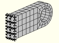
In the model of the connecting lug, all the nodes need to be constrained in all three directions at the left-hand end where it is attached to its parent structure (see Figure 4–19).
If you defined the boundary conditions in a preprocessor such as ABAQUS/CAE, each constrained degree of freedom is specified individually in the *BOUNDARY option block, as shown below:
*BOUNDARY
3241, 1,1
3241, 2,2
3241, 3,3
......
If a large number of nodes are constrained, these data can occupy a great deal of space in the computer's memory. Where a number of nodes all have the same boundary conditions, it is more efficient to apply the constraints directly to a node set containing all the nodes. Thus, in the lug model we prefer to create the node set LHEND to specify the constraints:
*BOUNDARY
LHEND, ENCASTRE
If you think that you defined the boundary conditions incorrectly, you can display them in ABAQUS/Viewer and compare them with the boundary conditions shown in Figure 4–19. The postprocessing instructions given at the end of “Postprocessing with ABAQUS/Viewer,” Section 2.7, discuss how to do this.
Loading
The lug carries a pressure of 50 MPa distributed around the bottom-half of the hole. Pressure loads can be defined conveniently using the preprocessor by selecting the element faces to which the load is applied. In the connecting lug input file, these loads will appear as a *DLOAD option block. For example, the *DLOAD option block for the connecting lug may look like
*DLOAD
   1,  P6, 5.E+07
   2,  P6, 5.E+07
   3,  P6, 5.E+07
   4,  P6, 5.E+07
  13,  P6, 5.E+07
...

1015,  P6, 5.E+07
1016,  P6, 5.E+07
The format of each data line is
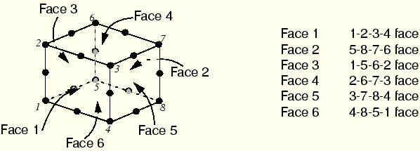
<element or element set name>, <load ID>, <load magnitude>In this case the “load ID” consists of the letter “P” followed by the number of the element face to which pressure is applied. The face numbers depend on the connectivity of the element and are defined for each element type in the ABAQUS Analysis User's Manual. For the three-dimensional hexahedral elements used in this example, the face numbers are shown in Figure 4–20.In the model, as defined in “Connecting lug,” Section A.2, the pressure is applied to face 6 of the elements around the bottom of the hole, so the load ID is “P6.”
For meshes generated with a preprocessor, the face numbers and, hence, the load IDs will depend on how the mesh is generated. Some preprocessors, such as ABAQUS/CAE, can determine the correct load ID automatically; this makes it very easy to specify pressure loads on complicated meshes. However, this method tends to produce long lists of data lines in the input file. In models where the same load ID and load magnitude are used for each element, you can use an element set—which is more efficient—to apply the pressure loads. For example, in this model the *DLOAD option block may appear as
*DLOAD
PRESS,  P6, 5.E+07
where we have made use of the element set PRESS whose members are shown in Figure 4–16.
Output requests
By default, many preprocessors create an ABAQUS input file that has a large number of output request options. These requests are in addition to the output database file request that is generated automatically by ABAQUS. If, when you edit your input file, you find that these additional output options were created, delete them because they will generally generate too much unnecessary output.
You were asked to determine the deflection of the connecting lug when the load is applied. A simple method for obtaining this result is to print out all the displacements in the model. However, it is likely that the location on the lug with the largest deflection is probably going to be on the bottom of the hole, where the load is applied. Furthermore, only the displacement in the 2-direction (U2) is going to be of interest. You should have created a node set, HOLEBOT, containing those nodes. Use that set to limit the requested displacements to just those five nodes at the bottom of the hole and to limit the output to just the vertical displacements.
*NODE PRINT, NSET=HOLEBOT
U2,
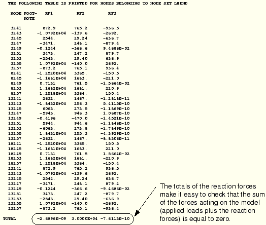
It is good practice to check that the reaction forces at the constraints balance the applied loads. All the reaction forces at a node can be printed by specifying the variable RF. We again use the node set LHEND to limit the output to those nodes that are constrained.
*NODE PRINT, NSET=LHEND, TOTAL=YES, SUMMARY=NO
RF,
You can define several *NODE PRINT and *EL PRINT options. The parameter TOTALS=YES causes the sum of the reaction forces at all the nodes in the node set to be printed. The SUMMARY=NO parameter prevents the minimum and maximum values in the table from being printed.
Add the following commands to print the stress tensor (variable S) and the Mises stress (variable MISES) for the elements at the constrained end (element set BUILTIN):
*EL PRINT, ELSET=BUILTIN
S, MISES
Indicate the end of a step with the option
*END STEPMake sure that this input option is the last option in your model.
Store the input in a file called lug.inp (an example file is listed in “Connecting lug,” Section A.2). Then, run the simulation using the command:
abaqus job=lug interactive
When the job has completed, check the data file, lug.dat , for any errors or warnings. If there are any errors, correct the input file and run the simulation again. If you have problems correcting any errors, try comparing your input file to the one given in “Connecting lug,” Section A.2. Check that you have the correct parameters for each input option.
When the job has completed successfully, look at the three tables of output that you requested. They will be found at the end of the data file. A portion of the table of element stresses is shown in Figure 4–21. The maximum Mises stress at the built-in end is approximately 306 MPa.
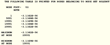
The tables showing the displacements of the nodes along the bottom of the hole and the reaction forces at the constrained nodes are shown in Figure 4–22 and Figure 4–23, respectively.
The bottom of the hole in the lug has displaced about 0.3 mm. The total reaction force in the 2-direction at the constrained nodes is equal and opposite to the applied load in that direction of –30 kN.Once you have looked at the results in the data file, start ABAQUS/Viewer by typing
abaqus viewer odb=lugat the operating system prompt.
Plotting the deformed shape
To begin this exercise, plot the deformed model shape.
From the main menu bar, select Plot![]() Deformed Shape; or use the
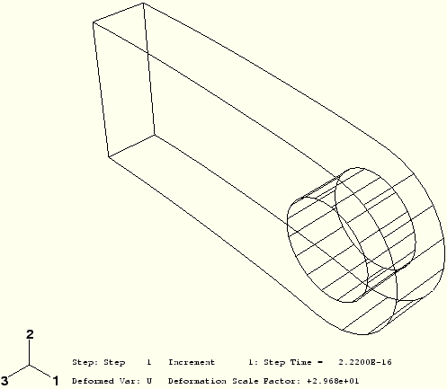
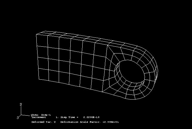
Deformed Shape; or use the ![]() tool in the toolbox. Figure 4–24 displays the deformed model shape at the end of the analysis. What is the displacement magnification level?
tool in the toolbox. Figure 4–24 displays the deformed model shape at the end of the analysis. What is the displacement magnification level?
Changing the view
The default view is isometric. You can change the view using the options in the View menu or the view tools in the toolbar.
To rotate the view:
From the main menu bar, select View![]() Rotate; or use the
Rotate; or use the ![]() tool from the toolbar.
tool from the toolbar.
Drag the cursor over the virtual trackball in the viewport.
The view rotates interactively. Try dragging the cursor inside and outside the virtual trackball to see the difference in behavior.
To specify the view:
From the main menu bar, select View![]() Specify.
Specify.
The Specify View dialog box appears.
From the list of available methods, select Viewpoint.
In the Viewpoint method, you enter three values representing the X-, Y-, and Z-position of an observer. You can also specify an up vector. ABAQUS positions your model so that this vector points upward.
Enter the X-, Y-, and Z-coordinates of the viewpoint vector as 1, 1, 3 and the coordinates of the up vector as 0, 1, 0.
Click OK.
ABAQUS/Viewer displays your model in the specified view, as shown in Figure 4–25.
Visible edges
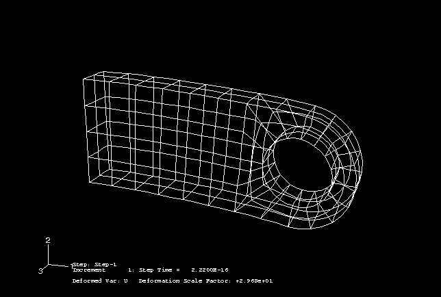
Several options are available for choosing which edges will be visible in the model display. The previous plots show all visible edges of the model; Figure 4–26 displays only feature edges.
To display only feature edges:
From the main menu bar, select Options![]() Deformed Shape.
Deformed Shape.
The Deformed Shape Plot Options dialog box appears.
Click the Basic tab if it is not already selected.
From the Visible Edges options, choose Feature edges.
Click OK.
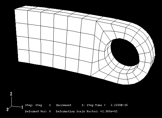
The deformed plot in the current viewport changes to display only feature edges, as shown in Figure 4–26.
Render style
A wireframe model showing internal edges can be visually confusing for complex three-dimensional models. Three other render styles provide additional display options: hidden line, filled, and shaded. You can select a render style from the Options menu on the main menu bar or from the render style tools on the toolbar: wireframe ![]() , hidden line
, hidden line ![]() , filled
, filled ![]() , and shaded
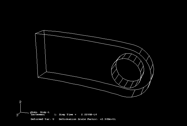
, and shaded ![]() . To display the hidden line plot shown in Figure 4–27, select hidden line plotting for the deformed plot mode by clicking the
. To display the hidden line plot shown in Figure 4–27, select hidden line plotting for the deformed plot mode by clicking the ![]() tool. Deformed shape plots will be displayed in the hidden line render style until you select another type of display.
tool. Deformed shape plots will be displayed in the hidden line render style until you select another type of display.
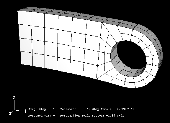
You can use the other render style tools to select filled and shaded render styles, shown in Figure 4–28 and Figure 4–29, respectively.
A filled plot colors the element faces a solid color. A shaded plot is a filled plot in which a lightsource appears to be directed at the model. These render styles can be very useful when viewing complex three-dimensional models.Contour plots
Contour plots display the variation of a variable across the surface of a model. You can create filled or shaded contour plots of field output results from the output database.
To generate a contour plot of the Mises stress:
From the main menu bar, select Plot![]() Contours.
Contours.
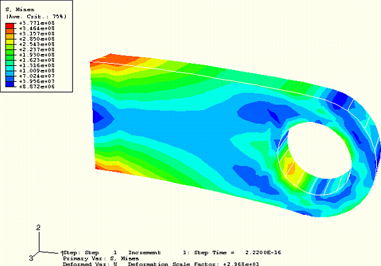
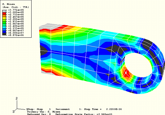
The filled contour plot shown in Figure 4–30 appears.
The Mises stress, S Mises, indicated in the legend title is the default variable chosen by ABAQUS for this analysis. You can select a different variable to plot.
From the main menu bar, select Result![]() Field Output.
Field Output.
The Field Output dialog box appears; by default, the Primary Variable tab is selected.
From the list of available output variables, select a new variable to plot.
Click OK.
The contour plot in the current viewport changes to reflect your selection.
ABAQUS/Viewer offers many options to customize contour plots. To see the available options, click Contour Options in the prompt area. By default, ABAQUS/Viewer automatically computes the minimum and maximum values shown in your contour plots and evenly divides the range between these values into 12 intervals. You can control the minimum and maximum values ABAQUS/Viewer displays (for example, to examine variations within a fixed set of bounds), as well as the number of intervals.
To generate a customized contour plot:
In the Limits tabbed page of the Contour Plot Options dialog box, choose Specify beside Max; then enter a maximum value of 300E+6.
Choose Specify beside Min; then enter a minimum value of 60E+6.
In the Basic tabbed page of the Contour Plot Options dialog box, drag the Contour Intervals slider to change the number of intervals to nine.
Click Apply.
ABAQUS/Viewer displays your model with the specified contour option settings, as shown in Figure 4–31. These settings remain in effect for all subsequent contour plots until you change them or reset them to their default values.
Maximum and minimum values
The maximum and minimum values of a variable in a model can be determined easily.
To report the minimum and maximum values of a contour variable:
From the main menu bar, select Viewport![]() Viewport Annotation Options; then click the Legend tab in the dialog box that appears.
Viewport Annotation Options; then click the Legend tab in the dialog box that appears.
The Legend options become available.
Toggle on Show min/max values.
Click OK.
The contour legend changes to report the minimum and maximum contour values.
Based on the contour legend in your plots, what is the maximum value of Mises stress in the model? How does it compare to the value reported in the data (.dat) file? Do the two maximum values correspond to the same point in the model? The Mises stresses shown in the contour plot have been extrapolated to the nodes, whereas the stresses written to the data file for this problem correspond to the element integration points. Therefore, the location of the maximum Mises stress in the data file is not exactly the same as the location of the maximum Mises stress in the contour plot. This difference can be resolved by requesting that stress output at the nodes (extrapolated from the element integration points and averaged over all elements containing a given node) be written to the data file. If the difference is large enough to be of concern, this is an indication that the mesh may be too coarse.
One of the goals of this workshop was to determine the deflection of the lug in the negative 2-direction. You will contour the displacement component of the lug in the 2-direction to determine its peak displacement in the vertical direction. In the Contour Plot Options dialog box, click Defaults to reset the minimum and maximum contour values and the number of intervals to their default values before proceeding.
To contour the displacement of the connecting lug in the 2-direction:
From the main menu bar, select Result![]() Field Output.
Field Output.
The Field Output dialog box appears; by default, the Primary Variable tab is selected.
From the list of available output variables, select U.
From the list of available components, select U2.
Click OK.
Displaying a subset of the model
By default, ABAQUS/Viewer displays your entire model; however, you can choose to display a subset of your model called a display group. This subset can contain any combination of part instances, elements, nodes, and surfaces from the current output database. For the connecting lug model you will create a display group consisting of the elements to which the pressure load was applied.
To display a subset of the model:
From the main menu bar, select Tools![]() Display Group
Display Group![]() Create.
Create.
The Create Display Group dialog box opens.
From the Item list, select Elements. From the Method list, select Element sets.
Once you have selected these items, the list on the right hand side of the Create Display Group dialog box shows the available selections.
From this list, choose element set PART-1-1.PRESS. Toggle on Highlight items in viewport below the list.
Note: A finite element model in ABAQUS can be defined as an assembly of part instances. For input files not written by ABAQUS/CAE, the use of part and assembly definitions in the input file is optional. However, since ABAQUS/Viewer displays results in terms of an assembly of part instances, an assembly and at least one part instance will be created automatically by the analysis input file processor if they are not defined in the input file. The prefix PART-1-1 is the default name given to the part instance in such a case.
The outlines of the elements in element set PART-1-1.PRESS are highlighted in red.
Click Replace to replace the current model display with the element set PART-1-1.PRESS.
ABAQUS/Viewer displays the specified subset of your model.
When creating an ABAQUS model, you may need to determine the face labels for a solid element so that you can determine the correct load ID when applying pressure loads or when defining surfaces for contact. If you use a preprocessor to generate the mesh, you may not be sure of the connectivity or orientation of the elements. In such situations you can use ABAQUS/Viewer to display the mesh after you have run a datacheck analysis that creates an output database file.
To display the face identification labels and element numbers on the undeformed model shape:
From the main menu bar, select Options![]() Undeformed Shape.
Undeformed Shape.
The Undeformed Plot Options dialog box appears.
Change the render style to filled since face labels cannot be displayed when the render style is set to wireframe; all visible element edges will be displayed for convenience.
Toggle on Filled under Render Style.
Toggle on All edges under Visible Edges.
Click the Labels tab, and toggle on Show element labels and Show face labels.
Click OK to apply the plot options and to close the dialog box.
From the main menu bar, select Plot![]() Undeformed Shape.
Undeformed Shape.
ABAQUS/Viewer displays the element and face identification labels in element set PART-1-1.PRESS.