| Joe Fiala (A paper written under the guidance of Prof. Raj Jain) |
Download |
As cloud computing has become more popular due to the efforts of big name companies such as Amazon, Google, and Microsoft, it has allowed for the amount of available data to increase exponentially [Li13][Bala14][Vinay15], leading to increased opportunities for utilization. As a result, cloud computing and machine learning (ML) have formed a partnership, of sorts, in which both benefit from the other's advancement and refinement. ML, for example, has been able to better train its algorithms from the increased datasets, leading to results such as Facebook's DeepFace - an algorithm that identifies faces and records accuracies of up to 97.35%. [Taigman14] For the purposes of this paper, however, the growth of machine learning from cloud computing will be put on hold in favor of discussing the particular applications offered to cloud computing by ML. In particular, the following paper will begin with a discussion on the ways in which ML can help to better predict and manage resources on virtual machines (VMs). From there, it will move to a look at ways in which ML can reduce energy consumption on servers and datacenters before concluding with an examination of the potential security benefits offered by ML. Finally, I conclude with a summary of the approaches discussed, citing their strengths, weaknesses, and areas for improvement, from which future research can expand upon.
Despite the prevalence of cloud computing, the most popular cloud vendors have yet to capitalize on dynamic resource management. Amazon, Google, and Microsoft each offer some degree of limited customizability for one's virtual instance - such as the ability to choose the number of cores, the amount of memory, and the capacity (and type) of storage. However, once configured, the virtual machine (VM) is static, meaning that if a customer requires more resources for their virtual machine, they must request more resources. Likewise, if a customer only uses 10% of their VM's resources, the rest essentially goes to waste and cannot be redistributed to other customers or used by the vendors for their own purposes. As a result, the following section will focus on recent work dealing on cloud resource prediction and management using ML in order to outline paths by which cloud vendors can offer more dynamic services effectively and reliably.
Of the recent work, the three most commonly cited approaches to dynamic resource management are linear regression (LR), support vector machine (SVM), and artificial neural network (ANN). Usually, LR is used as the baseline ML method from which the other two (SVM and ANN) are compared, in order to gauge their effectiveness and their potential advantages and disadvantages; however, sometimes LR is used in addition to the other proposed techniques in order to capture particular features produced by SVM or ANN. As a result, the bulk of the work done in this section will be focused on SVM and ANN.
In this section, we will first take a brief look at the ways in which SVM is implemented by both [Matsunaga10] and [Kundu12]. We will then see how each implementation fared, particularly in relation to an LR model, which the authors take as the baseline standard for comparison.
For SVM implementation, the focus is primarily on performing non-linear classification using a kernel function, which allows for effective mapping of inputs onto some multi-dimensional vector space [Matsunaga10][Kundu12]. Of the possible kernels, polynomial and radial basis functions prove to be the most popular, due to their ability to analyze input samples in relation to others, as well as their ability to analyze input samples in combination and compared to vectors of higher dimensionality. Once the classification is complete, LR is then used in order to construct a hyperplane from the mapping, thereby obtaining the final model from which the predictions for the appropriate VM are made.
In order to gauge how the SVM method performed, [Matsunaga10] and [Kundu12] used decidedly different environments. [Matsunaga10] decided to evaluate the models using two bioinformatics applications, Basic Local Alignment Search Tool (BLAST) and Randomized Axelerated Maximum Likelihood (RAxML). Additionally, [Matsunaga10] evaluated the models based on predicted required resources as well as predicted execution time, the results of which can be seen in Figure 1.
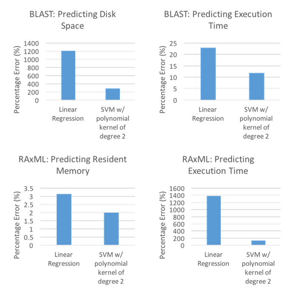
As Figure 1 shows, SVM is the victor in both predicted resources and predicted execution time for both the BLAST and RAxML environments. Moreover, SVM shows clear advantages in three of the four cases - BLAST: Predicting Disk Space, BLAST: Predicting Execution Time, and RAxML: Predicting Execution Time. In these cases, SVM reduces percentage error from 1204 to 283, 22.98 to 11.84, and 1379 to 135, respectively. Even in the case in which SVM does not show as clear of dominance, RAxML: Predicting Resident Memory, SVM still reduces percentage error down to 2.01 from 3.14 (via LR).
[Kundu12], on the other hand, decided to use two benchmark environments in order to test the generated SVM model, the Rice University Bidding System (RUBiS) and Filebench. In addition to the two global environments (RUBiS and Filebench), [Kundu12] supplemented the tests with the following additional sub-models in order to achieve finer granularity with regards to results for each test: RUBiS Browsing, RUBiS Bidding, Filebench OLTP, Filebench Webserver, and Filebench Fileserver. It is also important to note that unlike [Matsunaga10], [Kundu12] measured only predicted resources, rather than predicted resources and predicted execution time. The results of the tests can be seen in Figure 2.
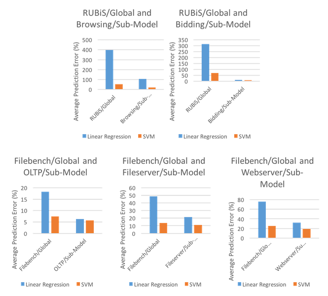
From the results, we can see that in all testing environments, SVM outperforms LR. However, we also see that the results are varied in terms of dominance. In both test cases using RUBiS, we see that SVM significantly outperforms LR in both the global and sub-model cases. However, in the Filebench test cases, such performance is not mirrored. In each of the Filebench/Global cases, we do see that SVM outperforms LR by quite some margin, but in each of the sub-model cases, the performance margin is much smaller and there may no longer be a clear benefit to using SVM over LR in such cases. Additionally, it's interesting to note that, overall, RUBiS presented much higher average percent prediction errors for both LR and SVM and for both the global model and sub-models, demonstrating an inability for either LR or SVM to find ample success using the RUBiS environment.
As we can see, both [Matsunaga10] and [Kundu12] find similar results when testing the performance of SVM as compared to LR in regards to resource prediction: namely, SVM clearly outperforms LR across most test cases. And even in those cases in which the gap between SVM and LR is not quite so large, the gap still does, in fact, exist, demonstrating a strict dominance of SVM over LR in the test cases examined, thus concluding our examination of SVM.
In this section, we will again visit the work by [Matsunaga10] and [Kundu12], but rather than discussing SVM, we will focus on ANN. We will begin by briefly examining the ways in which ANN is implemented before continuing on to the results obtained by both papers, as compared to the standard performance of LR.
For any ANN implementation, the focus is primarily on obtaining a balanced hidden neuron to hidden layer ratio, in order to avoid under-fitting from lack of weight or over-fitting from excess weight with regards to input. To obtain this balance, one could naively set a standard ratio and observe results for all tests using that ratio. [Matsunaga10] However, an alternative approach is to iteratively add more hidden neurons until no noticeable change in accuracy occurs, at which point more hidden layers are added. This is then repeated until neither additional hidden neurons nor additional hidden layers improve accuracy, thereby achieving a testable model with a more accurate balance [Kundu12].
Regardless of the implementation used, there needs to exist environments in which to test the models generated. We have seen that both [Matsunaga10] and [Kundu12] use the same environments for tests of ANN as for tests of SVM (as seen in 2.1) - BLAST/RAxML and RUBiS/Filebench, respectively. Additionally, the comparison will be to LR (also like in 2.1) in order to give a baseline standard for comparison. The results of [Matsunaga10] using ANN can be seen in Figure 3, and the results of [Kundu12] can be seen in Figure 4.
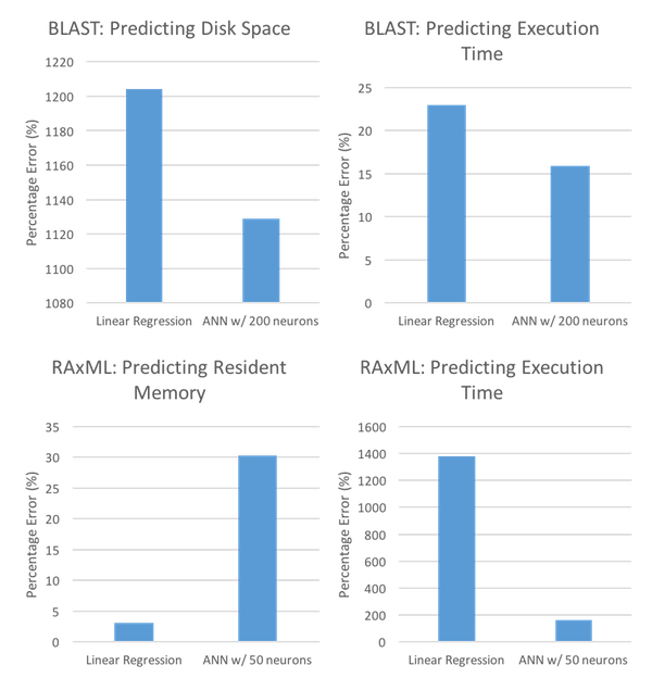
As Figure 3 shows, the results of ANN and LR are not nearly as one-sided as the results obtained while testing SVM and LR. That is, unlike SVM, which had the advantage over LR in both BLAST test cases and in both RAxML test cases, ANN performs better only in the BLAST: Predicting Disk Space case, BLAST: Predicting Execution Time, and the RAxML: Predicting Execution Time case. Even in the BLAST: Predicting Disk Space case, the performance is only marginally better (1129 compared to 1204) and still with an extraordinarily high percentage error. In RAxML: Predicting Resident Memory, however, LR performs significantly better, with percentage errors of 3.14 for LR and 30.29 for ANN, raising doubts about the superiority of ANN over LR.
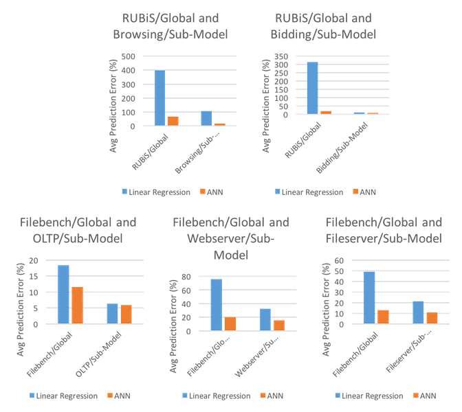
Unlike the results in Figure 3, the results in Figure 4 demonstrate a clear advantage for ANN over LR, demonstrating strict performance advantages in all test cases. Furthermore, in all cases except for Filebench/Global and OLTP/Sub-Model, ANN gives significantly better performance than LR, with less than half the average prediction error. And even in those cases in which ANN gives only moderate performance advantages, ANN keeps a relatively low prediction error, with rates of 12.89 and 10.60 for Filebench/Global and OLTP/Sub-Model, respectively. Also notable is that ANN never reaches the extremely high percentage error rates seen in Figure 3 (e.g. in BLAST: Predicting Disk Space, ANN had a 1129 percentage error rate) - in all tests performed by [Kundu12], the average prediction error was capped at 68.57, with the second highest average prediction error being 19.85.
Contrary to the tests involving SVM, [Matsunaga10] and [Kundu12] each achieved very different results. In [Matsunaga10]'s tests using BLAST and RAxML, ANN did not strictly outperform LR and in some cases performed significantly worse than LR. However, in [Kundu12]'s tests using RUBiS and Filebench, as well as their respective sub-models, ANN did strictly outperform LR and even in the cases in which ANN only outperformed LR marginally, ANN still achieved relatively low average prediction error rates.
Since we have seen implementations and results for both SVM and ANN, we can now turn to examining the comparison of SVM and ANN methods for those aforementioned test environments in [Matsunaga10] and [Kundu12]. We will first look at SVM and ANN in the BLAST and RAxML test cases, as seen in Figure 5, before turning to the RUBiS and Filebench test cases, as seen in Figure 6.
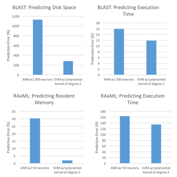
From the comparison in Figure 5, we can see that for all cases tested, SVM outperformed ANN. In the cases in which resources were predicted, SVM performed significantly better, with prediction errors of 283 and 2.01 compared to ANN's prediction errors of 1129 and 30.29. In the other cases, SVM only slightly outperformed ANN with prediction errors of 11.84 and 135 compared to 15.95 and 164. This demonstrates that although both performed relatively evenly in regards to predicting execution time, SVM was the clear victor in regards to the actual prediction of resources.
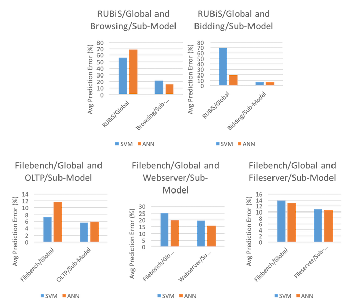
Unlike the results seen in Figure 5, the comparison in Figure 6 shows that SVM demonstrates no clear advantage over ANN in the RUBiS and Filebench test environments. Rather, there is only a single case in which either SVM or ANN shows clear superiority. In the RUBiS/Global and Bidding/Sub-Model case, the RUBiS/Global test showed that ANN outperformed SVM significantly, with average prediction errors of 19.52 and 66.86, respectively. In the only other notable cases, the average prediction errors slightly favored SVM, with error rates of 55.78 for SVM and 68.57 for ANN (in RUBiS/Global and Browsing/Sub-Model) and 7.4 for SVM and 11.59 for ANN (in Filebench/Global and OLTP/Sub-Model).
From what we have seen, it's hard to determine whether either SVM or ANN shows clear advantages over the other. If we were to only look at the test cases in [Matsunaga10], we might immediately judge that SVM clearly is the better method for dynamic resource management. However, the test cases in [Kundu12] demonstrate that SVM does not always perform significantly better than ANN, which highlights the importance of particular test environments in determining performance. That is, the preference of whether to use SVM or ANN for dynamic resource management may just come down to the particular environments and platforms a particular cloud vendor decides to use. For bioinformatics (as in [Matsunaga10]), SVM appears to be the clear winner; in other, more general applications (as in [Kundu12]), SVM and ANN appear to perform fairly equally.
In this section, we've taken a look at two proposed methods for dynamic resource management, SVM and ANN. In order to test these methods, a number of different environments were used and the results were first compared to the performance of LR in the same environment before finally comparing SVM to ANN for each environment. As a general rule, the results showed that both SVM and ANN outperformed LR except for a few outlying cases. However, it was less clear whether either SVM or ANN outperformed the other, with the conclusion seeming to be dependent upon the particular test environment in question. As a result, we can conclude that SVM and ANN are, in fact, more capable of predicting resources than LR, but the determination of SVM or ANN requires more testing for the particular scenario.
In addition to being able to better predict and allocate resources to the customer (as seen in section 2), being able to adaptively monitor, coordinate, and predict workload scheduling has become a key issue in terms of both quality of service (QoS) and energy efficiency (EE). That is, while it may be easiest to maintain an always active service in order to ensure that the service level agreement (SLA) between the vendor and company is always met (therefore maintaining a consistently high QoS), this always active server may require more energy than is absolutely necessary, leading to wasted resources. For example, if a customer is actively using the cloud resource in question every day from 9:00 AM to 5:00 PM, but never afterwards, it's not essential that the service be provided outside of the 9:00 AM to 5:00 PM range, thereby saving on resources that can be allocated to other customers (or back to the vendor, themselves), saving on costs of operation and maintenance, all while still maintaining the necessary QoS for the customer. In the following section, we'll look at some of the recent work being done in the fields of QoS and EE, starting with a more general overview of why such research is motivated, before considering the various approaches taken, and concluding with a summary of the approaches seen.
The essential focus of this section, more broadly, is to examine the ways in which dynamic and effective use of resources can be implemented, while still maintaining the necessary QoS. For the remainder of Section 3, the main points of focus will be on the following two techniques that can be utilized to save resources: (1) turning off idle machines; and (2) consolidation of tasks [Berral10].
Although these two techniques may seem trivial and obvious, their impact on energy consumption is enormous. In order to provide perspective into the issue of overall energy expenditure, [Berral10] recorded the results of wattage used in relation to increasing workload, as seen in Figure 7. These results were obtained using a 4-CPU and similarly results were previously observed by [Bianchini04].
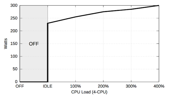
As we can see, Figure 7 demonstrates just how severe of an increase in energy is required for the shift between OFF and IDLE (0 Watts to 230 Watts), especially compared to the relatively modest shift between IDLE and the max CPU load of 400% (230 Watts to 300 Watts). With this in mind, the importance of turning off idle machines - in order to avoid the extreme energy requirements for the idle state - as well as the importance of consolidation - by allowing machines to be more fully utilized, thereby performing similarly to the max CPU seen above and allowing other machines to move to the off state, which saves energy overall - becomes more apparent. It is this importance that drives the motivation behind dynamic and effective use of resources, and will be key to understanding the research discussed later in this section.
In this section, we will focus on the work done by [Chase01], which uses a greedy algorithm, named Maximize Service Revenue and Profit (MSRP), in order to decrease power consumption in shared service centers. Although this research does not involve cloud computing, it provides a good basis from which further research into cloud computing EE can take place.
[Chase01] attempts to better determine the times in which energy is actually required, in order to avoid wasting energy for those times in which actual activity is minimal or nonexistent. With the typical static allocation of energy for a particular system, we see energy consumption compared to activity (throughput) similar to the mapping shown in Figure 8.
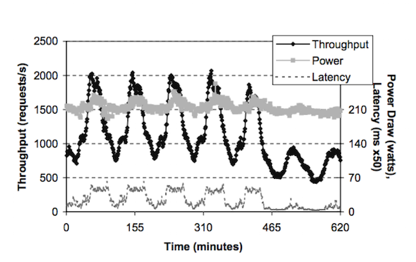
As we can see from Figure 8, the power consumption will remain fairly constant despite the activity fluctuating. This results in a massively inefficient use of energy - rather than always using the same amount of energy regardless, a more efficient use of the energy would have the energy consumption correspond to the rate of activity (i.e. more activity leads to more energy consumption).
In order to allow for this dynamic energy consumption, [Chase01] proposes MSRP. To construct the greedy algorithm, [Chase01] uses a weighted system involving resource costs, supplies, and demands. For each of these attributes, a weight is assigned, which is then used in order to determine prices for the resources. From these weights, resource prices are allowed to fluctuate according to the dynamically oscillating supply and demand for resources as well as the (potentially) dynamic resource costs. This weighting allows MSRP to allocate energy more efficiently than a simple, static allocation, as we can see in Figure 9.
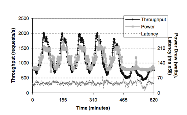
As we can see, MSRP allows for the energy consumption to vary according to the activity level - so when the activity level is low (e.g. minute 145), the energy consumption is also low; and when the activity level is high (e.g. minute 160), the energy consumption is also high. From this dynamic allocation, [Chase01] recorded an overall 29% savings of energy compared to the static allocation. However, it's also important to take note of the difference in latency levels between Figure 8 and Figure 9. In Figure 8 - the static allocation - we see latency levels that correspond to activity. However, in Figure 9 - the dynamic allocation - we see more consistent latency levels. In addition to the more static latency, the dynamic allocation appears to result in slightly higher overall latency levels than the static allocation.
As we have seen from [Chase01]'s greedy algorithm MSRP, a dynamic allocation of energy can result in overall savings in energy consumption. However, from the tests performed by [Chase01], this dynamic allocation resulted in a more consistent, and overall higher, level of latency than with the static allocation. As a result, any further research involving this dynamic allocation, or any customer wishing to use MSRP, would need to take into account both the potential benefits offered by the energy savings as well as the potential detriments of overall higher latency.
In this section, we will take a look at the work performed in [Berral10], in which a machine learning dynamic backfilling algorithm (MLDB) is used. In addition to MLDB, a variety of other algorithms will be considered, in order to best understand the advantages and disadvantages of MLDB. The other algorithms considered are as follows: random assignment, round-robin assignment, conventional backfilling, and non-machine learning dynamic backfilling. As the names of the algorithms suggest, the random assignment algorithm assigns tasks randomly, the round-robin assignment algorithm assigns tasks to all possible nodes evenly, the conventional backfilling algorithm attempts to assign a tasks in order to maximize individual node workload (thereby saving nodes from having to be utilized), the dynamic backfilling algorithm builds upon the conventional backfilling algorithm by also allowing task migration between nodes in order to increase consolidation, and the MLDB implements a supervised learning schema (as seen in Figure 10) and an SLA function in order to improve predictions and allow for better dynamic allocation.
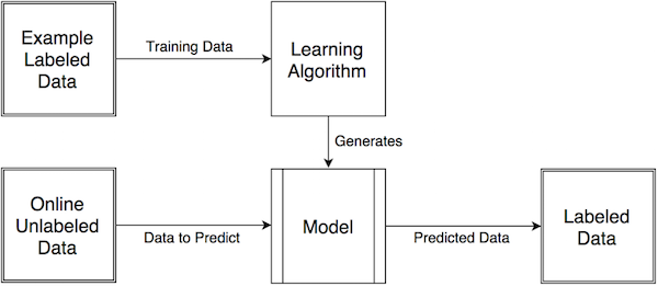
Essentially, the schema takes labeled data and feeds it into a particular learning algorithm (in this case, MLDB) in order to generate a model. With this model, we would then input unlabeled data and get labeled data as output. So as inputs for the MLDB model, we would feed in the characteristics of a particular scenario, involving data such as activity levels, energy consumption, SLA fulfillment, and so on.
In testing this particular method, [Berral10] found a key relationship between the aggressiveness of the turn on/off mechanism and the ability to fulfill the SLA - that is, the more cautious the turn on/off mechanism was, the easier it was to achieve higher SLA fulfillment. However, increased caution also resulted in higher energy consumption, due to leaving more machines idle or with less consolidation, leading to a tradeoff function. As a result, [Berral10] concluded that a compromise is best reached when λmin (earlier machine turnoff) and λmax (higher consolidation) have values of 30% and 60%, respectively, allowing for near complete SLA fulfillment while still retaining a sufficiently aggressive dynamic turn on/off mechanism to save energy.
To summarize the results obtained, the MLDB algorithm actually did not perform best in all cases, particularly in the case of grid workload, due to unnecessary caution. Although it achieved a 99.90 SLA fulfillment, it required 1574.78 kW of energy whereas the conventional backfilling algorithm and dynamic backfilling algorithm only required 1141.65 kW of energy and 1118.86 kW of energy, respectively. Furthermore, MLDB's energy consumption was only slightly better than the energy consumption of the round robin and random algorithms, which required 1696.66 kW of energy and 1671.16 kW of energy, respectively.
In the other two workload cases, however, MLDB did, in fact, perform better with regards to energy consumption. In the service workload, MLDB consumed roughly 3000 less kW of energy than either the conventional backfilling algorithm or the dynamic backfilling algorithm and roughly 6000 less kW of energy than either the round robin algorithm or random algorithm. Moreover, MLDB still managed to achieve 100.00 SLA fulfillment in the service workload.
Slightly less impressive, but still notable is that MLDB performed best with regards to energy consumption in the heterogeneous workload. MLDB consumed roughly 1000 less kW of energy than either the conventional backfilling algorithm or the dynamic backfilling algorithm and roughly 4500 less kW of energy than either the round robin algorithm or random algorithm. However, unlike the service workload, this decreased energy consumption comes at the cost of decreased SLA fulfillment. In the heterogeneous workload, MLDB achieved 98.63 SLA fulfillment, while conventional backfilling achieved 99.50 SLA fulfillment and dynamic backfilling achieved 99.59 SLA fulfillment.
From the results, it is clear that MLDB offers better performance than both the round robin algorithm and random algorithm, as expected. However, it is less clear whether MLDB should be preferred to either the conventional backfilling algorithm or the dynamic backfilling algorithm. On the one hand, MLDB has a clear performance advantage in the service workload and heterogeneous workload with regards to energy consumption. However, MLDB performs significantly worse in the case of grid workload. Furthermore, the advantage in the heterogeneous workload comes with the cost of slightly less SLA fulfillment than either conventional backfilling or dynamic backfilling (98.63 compared to 99.50 and 99.59). Ultimately, this allows us to conclude that MLDB is clearly better than the naive algorithms, round robin and random, but is only better than the conventional backfilling and dynamic backfilling algorithms under certain conditions, such as service workload and heterogeneous workload without extreme need for the difference in SLA fulfillment.
In each of the previous subsections, we have focused on broad approaches to energy efficiency. In this section, however, we will take a look at the work in [Chen13], which offers a more fine grained approach to determining energy efficiency in cloud computing. In order to do this, [Chen13] proposes using autoregressive moving-average model with exogenous inputs model (ARMAX) and ANN. In particular, the goal is to expand the traditional ARMAX and ANN algorithms to new sensitivity aware algorithms, sensitivity aware ARMAX (S-ARMAX) and sensitivity aware ANN (S-ANN), in order to obtain the highest possible QoS with the minimal energy expenditure by capturing the sensitivity on inputs for more fine grained results.
In order to measure the results obtained by each of the algorithms in a more fine grained way, [Chen13] focused on three particular attributes: (1) availability; (2) response time; and (3) throughput. The results are compiled together in Table 1, in which the two newly extended ML algorithms, S-ANN and S-ARMAX, are compared to the conventional ML algorithms, ANN and ARMAX.
|
Symmetric Mean Absolute Percentage Error of Prediction |
||||||
|
QoS |
S-ANN |
ANN |
S-ARMAX |
ARMAX |
||
|
per-service |
per-application |
per-service |
per-application |
|||
|
Response Time |
6.97% |
12.76% |
31.72% |
11.43% |
15.08% |
34.03% |
|
Throughput |
11.14% |
16.88% |
35.28% |
7.99% |
13.22% |
37.82% |
|
Availability |
0.96% |
0.38% |
1.36% |
0.01% |
0.01% |
1% |
From Table 1, we can see that both S-ANN and S-ARMAX offer clear advantages to both ANN and ARMAX, respectively in regards to response time and throughput and perform on par with ANN and ARMAX in regards to availability, depending on whether ANN and ARMAX are run per-service or per-application. Indeed, even when only running per-service, both S-ANN and S-ARMAX clearly outperform their conventional counterparts. For example, in regards to response time, S-ANN's error of prediction was 6.97 whereas ANN's error of prediction was 12.76 per-service (and 31.72 per-application); likewise, S-ARMAX's error of prediction was 11.43 whereas ARMAX's error of prediction was 15.08 per-service (and 34.03 per-application.
In comparing the two sensitive aware algorithms, however, there is no clear winner. While S-ANN outperforms S-ARMAX in terms of response time (6.97 compared to 11.43), S-ARMAX outperforms S-ANN in terms of throughput and availability (7.99 compared to 11.14 and 0.01 compared to 0.96, respectively). This demonstrates that S-ARMAX appears to perform better in conditions with more stable QoS, whereas S-ANN performs better in more dynamic conditions, with a more volatile QoS.
As a result of the fine grained approach adopted by [Chen13], the advantages and disadvantages of the particular algorithms in question become more clear. While ANN and ARMAX offer the best error of prediction for availability per-service, they perform worse than S-ANN and S-ARMAX for availability per-application and worse than S-ANN and S-ARMAX for response time and throughput for both per-service and per-application. However, the decision of implementing S-ANN or S-ARMAX is more difficult and is dependent upon the particular conditions at hand. For more dynamic conditions, S-ANN performs better, and for more stable conditions, S-ARMAX performs better.
In this section, we've looked at a variety of approaches that aim to reduce overall energy consumption while maintaining sufficient QoS and SLA fulfillment by either turning off idle machines or by consolidating work among machines (in order to turn off idle machines). We started by looking at the greedy algorithm implemented by [Chase01], which provided a more dynamic mapping of energy consumption to activity level and demonstrated an overall 29% decrease in energy consumption. We then looked at a number of backfilling algorithms and compared them to naive algorithms like random assignment and round robin assignment. We saw that, generally, the backfilling algorithms outperformed the naive algorithms, but it was unclear whether the proposed algorithm, MLDB, was superior to the other two backfilling algorithms, conventional backfilling and dynamic backfilling, due to their performance being dependent upon particular conditions. This then motivated an examination of a more fine grained study of algorithms, for which we turned to [Chen13], in which ARMAX and ANN algorithms were used and measured in regards to a number of characteristics, where we saw that for more dynamic conditions, S-ANN performs better, where for more stable conditions, S-ARMAX performs better.
In this section we'll step away from the discussions about resource allocation (as seen in sections 2 and 3) and focus, instead on the ways in which ML can aid in the security of cloud computing. With the increase of overall data in the cloud, there has also been an increase of sensitive data in the cloud, motivating the need for higher security in cloud computing [Whitworth14]. This section will serve as an examination of various approaches proposed to improve cloud security via better threat detection. We will first start with a general approach in which to determine threats via summation of risk levels. We will then move to more advanced approaches to determine threats which make use of signature detection and anomaly detection in order to produce a hybrid model for threat detection.
In terms of encryption, one of the most straightforward ways to enable or deny access within the cloud is to enforce some system of trust levels. In such a system, trust levels are dynamically allocated to any participant within the cloud system and their privileges are assigned according to their determined trust level.
One such trust level algorithm is given in [Whiteworth14], in which the trust level is just a summation of all risk levels associated with the particular relationship in question, as seen in Equation 1 (with β representing the overall trust level and α representing the risk associated with each particular characteristic implicit in the relationship).

For each particular risk, α, the total risk associated with that characteristic is then calculated by having a weighted value, w, multiplied by the mitigation level, c, thereby producing a risk value that is weighted by importance as well as potential consequences, as we see in Equation 2.

By using this calculation of risk level, and in conjunction with the calculation of overall trust level via summing risk levels, each agent in the cloud is able to be associated with a particular degree of trust, thereby enabling privileges for that particular agent in addition to restricting access for that particular agent to certain features of the cloud.
In this section, we've taken a brief look into one way in which trust level can be calculated, namely via some general algorithm with weighted values for particular attributes that are then combined in order to produce an overall trust level. However, moving forward this offers very little advice and can become overly cumbersome in a complex environment in which characteristics are not necessarily known beforehand and therefore are not capable of being assigned a reliable weight.
To fix this, we can turn to two other methods, named signature detection and anomaly detection. In signature detection, agents are identified by their particular signature - as a result, intruders or other malicious agents are easily identified as potential risks if they have a history of malicious activity. However, signature detection is limited in that it is generally unable to detect threats whose signatures have not yet been identified [Bhat13][Gander13]. As a result, anomaly detection is often used. Anomaly detection determines potential risks based on an agent's deviation from standard behavior, thereby painting it as an "anomaly" (and therefore a potential threat). The disadvantage to anomaly detection is that it suffers from a high false positive rate, in which it identifies particular benign agents as malicious [Bhat13]. Consequently, the two methods - signature detection and anomaly detection - are often used in conjunction to create a hybrid approach in which malicious signatures are detected and stored (for use in repeat and static circumstances) and anomaly detection is used for more dynamic situations (where signature detection has no data).
In this section, we will focus on a hybrid method for threat detection that makes use of Naive Bayes Tree (NBT) and Random Forest (RF), as outlined in [Bhat13]. The idea behind this approach is to first generate a classification pattern from training sets and then determine anomalies based on the classification pattern and similarity of features for each connection in the classification. As a result, we require extensive data sets in order to generate an accurate classification. To resolve this issue, [Bhat13] used data from the KDD Cup '99 data set [KDD09]. Additionally, the dataset was divided into subclasses based on the particular type of attack, as seen in Table 2.
|
Class of Attack |
Attacks in Dataset |
|
Probe |
Ipsweep, Nmap, Portsweep, Satan |
|
Denial of Service (DoS) |
Back, Land, Neptune, Pod, Smurf, Teardrop |
|
User to Root (U2R) |
Buffer_overflow, Loadmodule, Perl, Rootkit |
|
Remote to Local (R2L) |
Ftp_write, Guess_passwd, Imap, Multihop, Phf, Spy, Warezclient, Warezmaster |
From this dataset, [Bhat13] proposed to implement their method via use of both front-end and back-end processing, as seen in Figure 11. Essentially, the front-end is used to do the necessary pre-processing in addition to basic feature construction in order to accommodate (1) those algorithms which require pre-processing; and (2) those algorithms that require an already constructed feature set. On the back-end, the features are then reduced in order to create models, which are used to signal the anomaly detection system, which, in turn, signal the alarm for an intruder.
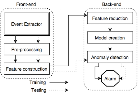
After the learning stage (which used the KDD datasets), [Bhat13] tested the model and measured performance based on percent accuracy and false positive rate. The model was then compared to the performance of a similar, competing model, which uses RF and K-Nearest Nodes (KNN) algorithms. The results of both models are displayed in Table 3.
|
Classifier |
Accuracy |
False Positive |
|
NBT + RF |
99.0% |
2.0% |
|
RF + KNN |
94.7% |
12.0% |
From the results, we can clearly see that the proposed method, using both NBT and RF, obtains better results both in regards to accuracy (99.0 to 94.7) as well as false positive rate (2.0 to 12.0). It is important to note that not only does the proposed method reduce the false positive rate, it does so dramatically; this is particularly important given the high false positive rate implicit in anomaly detection and demonstrates a significant step forward for any method planning on using anomaly detection for threat detection. However, it is also important to note that although the proposed method outperformed the RF and KNN method, [Bhat13] failed to compare the results to a wider variety of competing methods. This could have been due to a lack of competing methods or else a lack of relevance between the competing methods and the proposed methods, but is nonetheless unfortunate and is important to note.
In this section, we took a brief look at one way in which a hybrid method for threat detection could be constructed that made use of both signature detection and anomaly detection. More specifically, the method proposed by [Bhat13] uses NBT and RF in order to generate a classifier, from which we are able to better determine anomalies. We have also seen that this method improves upon already existing methods that rely solely on RF and KNN, but do not have sufficient data to make further conclusions about the performance of the proposed method compared to other ML algorithms.
In this section, we will focus on a proposed framework as seen in [Gander13] that emphasizes the identification of semantic gaps and anomalies in order to detect threats. Specifically, we will look at the ways in which semantic gaps are proposed to aid in threat detection as well as the process by which one may make conclusions from such a framework.
In order to detect semantic gaps, and therefore identify potential anomalies and threats, one must first specify a particular domain specific language (DSL) in which to work. The DSL is imperative, since it is used to better base the results generated by signature detection and anomaly detection, via specified workflows and monitoring rules present in the DSL. Once the DSL has been specified, the rules generated by the DSL allow for easier detection of semantic gaps, since such rules specify the necessary information in order to identify agents, allowing for signature detection to more correctly identify particular agents as malicious or benign.
From here, anomalies can be detected using ML techniques by taking advantage of the particular profiles gathered by the workflow by dividing each profile into four categories: (1) service; (2) user; (3) host; and (4) workflow. Each sub-profile is then used in order to gain insight as to the nature of the potential behavior associated with that particular sub-profile. Service profiles, for example, are used to determine fluctuations in activity as compared to past history and other profiles, whereas user profiles are used in order to monitor specific behavior, more generally, in order to prevent data theft [Gander13].
Going even further, each sub-profile can be further divided into particular time tracks: immediate, hourly, or monthly. Each of these time tracks allows for further classification of profiles, and allow for detection of anomalous behaviors not just in relation to other profile, but in relation to other profiles over time as well as one's own profile over time, issues which may not have been adequately handled by the model presented by [Bhat13].
Once these profiles have been gathered and classified, they can be analyzed via the clustering of fingerprints. Such a clustering essentially maps all of the particular profiles (and each of the profile's particular characteristics) and then compares each feature of each profile to the general cluster(s) formed. Outliers are then detected using some form of the Euclidian metric as seen in Equation 3 (by using each fingerprint to create a vector, v).

Moreover, in this model, once the outliers have been detected, the model can then make further relations among the outliers. This allows for the model to better learn potential threats (by connecting patterns among threats) as well as (hopefully) decreasing the rate of false positives by potentially finding connections among benign outliers that successfully identify such outliers as benign, due to some particular characteristic that the malicious profiles, in fact, contain.
Unfortunately, however, the model proposed in [Gander13] was just proposed as a framework and so had not been fully implemented or tested, either in isolation or in relation to other, competing methods. Nevertheless, the framework outlined in this section offered further insight as to how the currently implemented methods may improve their models via further specificity, either by reducing their framework to a particular DSL in order to identify semantic gaps or else by storing and classifying subdivisions of data corresponding to characteristics similar to profile type and/or time frame.
In this section, we have looked at the various proposed methods for detecting threats in cloud computing. We first started with a general algorithm, which provided a guideline for how threats could be determined by a calculated trust level via various risk levels. From this, we then turned to a proposed method in which NBT and RF were used, in conjunction with an already available dataset, in order to train a model to detect anomalies. And although this model outperformed another, competing model, further comparison was not made to other models, leaving the strength of the proposed method a bit questionable. Finally, we turned to a proposed framework by which threat levels can be better determined by narrowing the scope of focus to a specific DSL. Once this is done, we can then add specificity by having particular profile categories and time frames in order to better classify the profiles and detect anomalies. Consequently, while there is no clear method for security in cloud computing, the proposed models provide promising starting points for future work and offer insights as to the ways in which future work might proceed with regards to implemented algorithms and scope of specificity.
In this paper, we have looked at a variety of ways in which ML applications can be used to improve cloud computing. We started by looking at ML techniques for dynamic resource management, with particular focus on predictions of required VM size. We found that the two proposed techniques, SVM and ANN, both outperformed LR in most cases, and the determination of which of the two methods to use is situation dependent. We then turned to look at ML techniques for more efficient use of resources, particularly in order to save energy, by turning off idle machines and consolidation of workloads. Here, we again found that although the proposed methods outperformed the naive approach(es), choosing between the proposed methods required further specificity that is situation dependent. Finally, we concluded with a discussion of security in cloud computing. We started with a generic algorithm for determining trust levels, from which more advanced techniques could build upon. One such technique, using NBT and RF, demonstrated improved performance but was not adequately compared to other methods in order to achieve a decisive conclusion. Another technique was proposed merely as a framework and so was not able to be tested, but nevertheless offered intriguing perspectives for future work to build upon.