Performance Measurement of BLAST as a MERCATOR Application

Stephen Timcheck, stimcheck (at) wustl (dot) edu (A paper written under the guidance of Prof. Raj Jain)

Download

Abstract

With the increase in parallel computing applications, there has been a need to construct libraries which support said applications. MERCATOR is a framework running on NVIDIA CUDA which aims to make constructing applications for GPUs more easy. This study examines the overhead incurred from MERCATOR in MERCATOR applications and how they effect execution time. We found that changing the topology of the MERCATOR application does indeed effect the execution time of the application.

Table of Contents

• 1. Introduction
• 2. Background
  • 2.1. SIMD Parallelism
  • 2.2. MERCATOR Overview
  • 2.3. BLAST Overview
• 3. Experimental Design
  • 3.1. System Definition
  • 3.2. Services
  • 3.3. Metrics
  • 3.4. System Parameters
• 4. Evaluation Technique
• 5. Performance Study
  • 5.1. Results
  • 5.2. Analysis
• 6. Conclusion
• 7. Future Work
• References
• Acronyms

Keywords: General Purpose GPU Programming, MERCATOR, BLAST, SIMD, Performance Evaluation, Data Flow, CUDA, Overhead

1. Introduction

With the ever increasing amount of data in the world, applications need to be able to sift through information to determine what is and is not important. One such route developers have taken is to utilize parallelism to acquire relevant data or calculate meaningful information from vast quantities of data. In particular, the use of parallel computing platforms such as GPUs have become a popular means of utilizing big data [NVIDIA17a]. In this experiment, we explore the usage of NVIDIA GPUs with CUDA using the MERCATOR framework and how the overhead of said framework effects performance.

2. Background

Parallel computing can take many paradigms including MISD, MIMD, and SIMD [Ghosh06].

2.1. SIMD Parallelism

SIMD stands for Single Instruction Multiple Data. By definition, SIMD processors apply a single instruction to multiple data points at once [Ghosh06]. For example, a processor wants to increment all data points in an array by 1. If the processor uses the SIMD paradigm, then the processor only needs to execute a single instruction, an addition of 1, which will apply to all entries in the array. By comparison, most modern day consumer processors are SISD processors, or single instruction single data, perform a single instruction on a single entry at a time. In the previous example, the SISD processors would need to increment each entry by 1 individually. The difference in execution is shown in Figure 1. In this experiment, we utilize a SIMD processor in the form of NVIDIA GPUs.

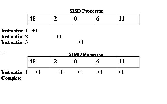
Figure 1: SISD vs. SIMD Processor Model

GPUs, or Graphics Processing Units, are designed for graphics applications as the name would imply and use a SIMD processing model. These processors have multiple cores working on different entries at the same time using the same instruction. For our tests, we used the CUDA architecture, a group of libraries for implementing general purpose applications for NVIDIA GPUs [NVIDIA17b].

2.2. MERCATOR

MERCATOR is a framework for building applications on the GPU using CUDA developed by Dr. Stephen Cole. The framework is designed for creating an easy way for developers to construct efficient implementations of irregular data applications, which are not commonly well supported on GPUs. Irregular data applications as defined by Dr. Cole are ,"... applications that exhibit some form of divergent control flow, unbalanced workloads, unpredictable memory accesses, input-dependent dataflow, and complicated data structure requirements," [Cole 17].

To represent these types of applications, MERCATOR uses Data Flow Graphs. A graph of a typical application is shown in Figure 2.

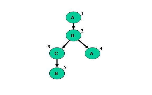
Figure 2: MERCATOR Data Flow Graph

These graphs represent the application through nodes, modules, and edges. Nodes are parts of the application where operations are performed by the GPU. The code each node executes is dictated by what module they are. In the example above, the first node is of type Module A, the second and fifth are of type Module B, the third is of type Module C, and the fourth is also of type Module A. All the nodes of the same module run the same code, but may have different inputs depending on where they exist in the graph. Finally, the edges connect the nodes together and define what kind of and how much data travels across it.

2.3. BLAST

BLAST, or Basic Local Alignment Search Tool, is an application developed for DNA sequence comparison [Altschul90]. Many implementations have been made of this application due to its high impact in the field of Genomics, the most notable being NCBI-BLASTN. Various other groups have used GPUs to accelerate BLAST such as GPU-BLAST with a speedup from NCBI-BLAST ranging from 3 to 4 on average [Vouzis11].

However, many of the GPU accelerated implementations for BLAST are only built for BLAST. That is, many of the same design ideas utilized in the construction of BLAST could be used to develop other irregular data flow applications. This is why we would like to see the viability of MERCATOR as a general purpose framework for producing efficient high impact applications such as BLAST on GPUs.

BLAST can be partitioned into 4 modules in MERCATOR: Seed Matching, Seed Enumeration, Small Extension, and Ungapped Extension. The application graph for MERCATOR is shown in Figure 3 below.

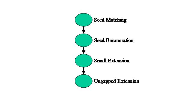
Figure 3: BLAST application graph in MERCATOR

First, the Seed Matching module takes multiple database strings, in this case 8 DNA bases, and compares them to a hash table of the query string. This stage determines whether or not the database sequence exists anywhere in the query sequence.

Second, the Seed Enumeration module takes the database sequences that exist in the query and determines how many instances of the match exists between the two. For example, a database string exists in two places in the query. This stage will know that the match exists from the prior stage and will iterate over all the instances where the match occurs. All the matches found will then be sent off to the next stage as points, with starting positions in the query and database.

Next, the Small Extension module extends the points found earlier to include the next 3 bases to first the left, then the right. If either side of the extension matches, then the match passes to the following stage.

Finally, the Ungapped Extension module performs a user defined window size extension on the match. This extension is the same as the previous module, but extends for however long the user defines, in our case 64 bases to the left and 64 bases to the right. Matches are given a score of +1 and mismatches a score of -3. The module then determines if the maximal score at any point in the matching process is greater than a user defined value and either discards the match, or stores the match to be returned to the CPU side of the application for further processing.

From domain knowledge, we know that as the data moves through the BLAST pipeline of execution, the amount of data shrinks and the execution time increases [Cole17]. Thus, it should be advantageous to separate all the stages assuming there is no overhead. For our tests, we would like to see whether or not the overhead of MERCATOR is worth splitting all the stages into separate modules, or if a unified module containing all the separate module code or some mix of the two is most optimal for execution time.

3. Experimental Design

In this section, we will discuss the design of the experiment. We will first explore the system definition and then describe the services, metrics, and parameters of the system. We then will explore which factors we wish to learn more about.

3.1. System Definition

The system under exploration is a MERCATOR application implementing the BLAST pipeline described in section 2.3. The study will examine the performance implications of MERCATOR overhead in the BLAST pipeline.

3.2. Services

The system described offers a single service, finding matches between query and database strings of DNA bases. As outlined in section 2.3, the BLAST pipeline takes a query string and database string of DNA bases, and provides the user with the points in the files which match the best.

3.3. Metrics

For this study, we will examine 2 factors:

• Model Type
• Workloads

Model Type will have 3 levels:

• Unified
• Separate
• Mixed

Workloads will have 2 levels:

• Small
• Large

3.3.1. Model Type

The Model Type describes the topology of the current experiment. As described in section 2.3, there are 4 modules that exist in the BLAST pipeline. To determine how to properly combine modules to minimize execution time, we will examine 3 types of application topologies for BLAST.

The first topology is Unified. This topology has all of the modules combined into one module. The application graph is shown below in Figure 4. We expect this model type to have the worst performance for this application.

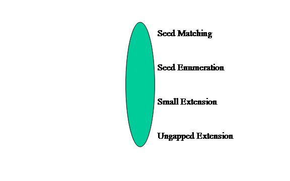
Figure 4: Unified Model Type of BLAST application

The third and final topology is Mixed. Given that we know from domain knowledge that the Seed Matching stage filters out almost all non-matches, as well as has the shortest execution time, we will keep Seed matching in a separate node. The rest of the pipeline will remain combined as one node in the application graph as shown in Figure 5. We expect this model type to potentially have performance gains over the Separate model type due to having less overhead from infrequently executed later pipeline stages.

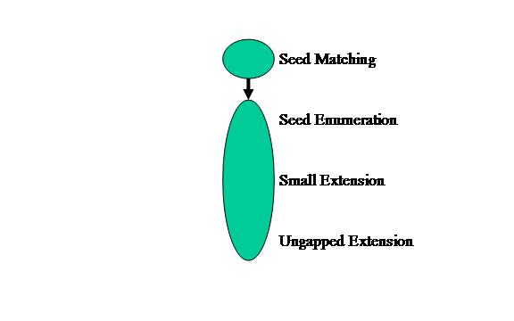
Figure 5: Mixed application graph

3.3.2. Workloads

The workloads are two text files containing DNA bases for the application. The application is built to use 2-bit data representations for the database string and a FASTA format (ASCII Characters) for the query string. The Small workload uses a 2KB portion of the salmonella genome as a query and a 2-bit representation of the human chromosome 1 for the database. The Large workload uses a 100KB portion of the salmonella genome as a query and a 2-bit representation of the human chromosome 1 for the database.

3.4. System Parameters

Parameters that could effect the system include:

• Model Type
• Workload
• GPU Architecture
• Graphics Card Specifications
• Thread to Work Mapping

For the purposes of this experiment, we can ignore the Graphics Card Specifications and Thread to Work Mapping. The first can be ignored since we will only be using a single GTX980Ti graphics card for testing. In addition, we can ignore the Thread to Work Mapping as we will only be testing work mapped 1 to 1. This means each thread in the GPU will only be performing operations on a single data entry at a time. We will also ignore the GPU Architecture as the application has been developed independent of the architecture.

4. Evaluation Technique

We define our experiment as a Two Factor Full Factorial Design with Replications. This design will utilize the two factors described in section 3.3, with Factor A being the Model Type and Factor B being the Workload. We will be using 5 replications of each combination to bring the total number of experiments to 30. We will be looking at the total execution time on the GPU of each combination. In addition, since we are examining execution time, we know that the model is multiplicative, and thus must perform a log transformation to attain accurate results [Jain91].

5. Performance Study

In this section, we will discuss our results and analysis of the execution times for the BLAST pipeline in relation to Model Type (A) and Workload (B).

5.1. Results

For the results we found each replication measured in Milliseconds (ms) to be as follows in Table 1:

Table 1: Measured Results

We then perform a log transformation on the dataset since we are examining execution times [Jain91]. Table 2 shows the results after the log base 10 transformation.:

Table 2: Log Base 10 Transformation on Measured Data

Next, we determine the effects of the Model Types and Workloads in Table 3:

Table 3: Effects of Model Types and Workloads

Now, we must calculate the effects of the interactions between the Model Types and Workloads in Table 4:

Table 4: Interactions between Model Types and Workloads

Then, we construct the ANOVA Table for the experiment:

Table 5: ANOVA Table

Next, we determine the 90% confidence intervals for the Model Types and Workloads in Table 6:

Table 6: 90% Confidence Intervals of Model Types (Alpha) and Workloads (Beta)

Likewise, we determine the 90% confidence intervals for the interactions between the Model Types and Workloads in Table 7:

Table 7: 90% Confidence Intervals of Interactions

Finally, we utilize visual tests to ensure that ensure that our experimental model is valid. We first verify if the errors are normally distributed with a QQ-plot in Figure 6:

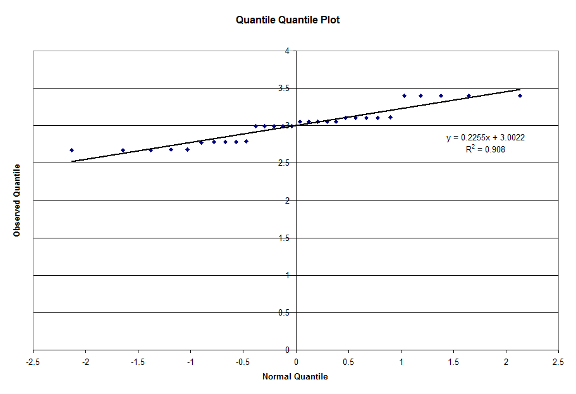
Figure 6: Quantile Quantile Plot

Lastly, we determine if the errors are independent with a plot of Residuals versus Predicted Responses in Figure 7:

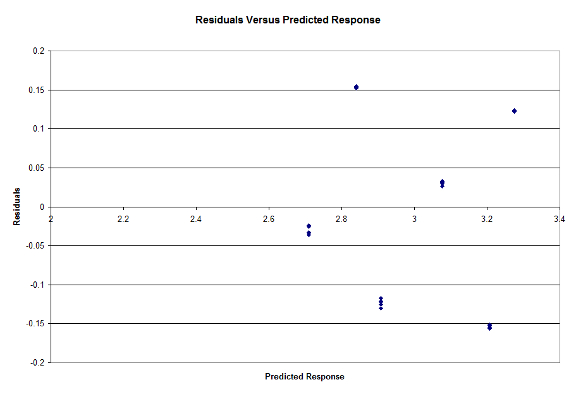
Figure 7: Residuals Vs Predicted Response

5.2. Analysis

From looking at the results, we can see that our hypothesis that the Mixed model type performed the best for the Small workload. For the Large workload however, we expected a result similar to what we achieved. Since the Large workload would contain the most number of matches between the database and query, the model with the least overhead would perform the fastest, hence why the Unified model runs the fastest [Cole17]. We have also determined that the Workloads and Model Type are significant factors at 90% Confidence, and our experiments pass the F-Test. From Figure 6, we can see that our data is normally distributed and from Figure 7 we see that the errors are independent. We have also determined that the Workload explains most of the variation in the model, and is thus the most important factor in the study. The Model type could also be considered important, but is nowhere near the importance of the Workload.

6. Conclusion

Through this study, we explored the effects of the overhead incurred when using MERCATOR. We found that in the Small case that our hypothesis of the Mixed implementation performing the best was true. However, the Large test case resulted in the opposite conclusion, showing the Unified implementation having the greatest performance. As mentioned before, this was the expected result, as almost all of the data would not be filtered by each filter, making the sparseness of the data in the final filters irrelevant to performance.

7. Future Work

Looking forward, we would like to determine where the threshold of the MERCATOR framework becomes detrimental to performance. Although we may have obtained a contradictory result between the Small and Large data sets, it still gives insight into what could be tested for future overhead in applications such as BLAST in the MERCATOR framework. It would be interesting to see if one could determine the overhead costs in relation to the total execution time to allow users to properly reconfigure their code, potentially automatically, to minimize total execution time for most cases.

References

[Altschul90] S. Altschul et al., "Basic Local Alignment Search Tool," Academic Press Limited, pp403-410, 1990, https://www.scribd.com/document/266260951/Basic-local-alignment-search-tool

[Cole17] S. Cole, J. Buhler, "MERCATOR: A GPGPU Framework for Irregular Streaming Applications," 2017 International Conference on High Performance Computing & Simulation (HPCS), 2017, pp727-736, http://ieeexplore.ieee.org/document/8035150/

[Ghosh06] "Multiprocessors," A presentation on Flynn's Classification of multiple-processor machines, http://homepage.divms.uiowa.edu/~ghosh/4-6-06.pdf

[Jain91] R. Jain, "The Art of Computer Systems Performance Analysis: Techniques for Experimental Design, Measurement, Simulation, and Modeling," Wiley-Interscience, New York, NY, April 1991, ISBN:0471503361.

[NVIDIA17a] "GPU Applications," A portal to various consumer applications using CUDA, http://www.nvidia.com/object/data-science-analytics-database.html

[NVIDIA17b] "Cuda C Programming Guide," Developers toolkit for CUDA introduction, http://docs.NVIDIA.com/cuda/cuda-c-programming-guide/#axzz4cZZhMRHt

[Vouzis11] P. Vouzis, N. Sahinidis, "GPU-BLAST: using graphics processors to accelerate protein sequence alignment," Bioinformatics, Volume 27, Issue 2, 2011, pp182-188, https://academic.oup.com/bioinformatics/article/27/2/182/285951

Acronyms

BLAST: Basic Local Alignment Search Tool
CUDA: Compute Unified Device Architecture
MERCATOR: Mapping Enumerator
GPU: Graphics Processing Unit
CPU: Central Processing Unit
SISD: Single Instruction Single Data
SIMD: Single Instruction Multiple Data

Last Modified: December 15, 2017
This and other papers on latest advances in Performance Analysis and Modeling are available on line at http://www.cse.wustl.edu/~jain/cse567-17/index.html
Back to Raj Jain's Home Page