| Samual B. Powell, s.powell@wustl.edu (A paper written under the guidance of Prof. Raj Jain) |
Download |
Division-of-focal plane (DoFP) imaging polarimeters are useful instruments for measuring polarization images for a variety of applications, however only recent advances in nanofabrication have enabled the practical manufacture of these sensors. These sensors are made by integrating nanowire polarization filters directly with an imaging array, and size variations of the nanowires due to fabrication can cause the optical properties of the filters to vary up to 20% across the imaging array. If left unchecked, these variations introduce significant errors when reconstructing the polarization image. Calibration methods offer a means to correct these errors. This work evaluates a scalar and matrix calibration derived from a mathematical model of the polarimeter behavior. The methods are evaluated quantitatively with an existing DoFP polarimeter while varying illumination intensity and angle of linear polarization.
Keywords: polarization, polarimeter, division-of-focal-plane, scalar calibration, matrix calibration
Polarization, along with intensity and wavelength, is one of the fundamental properties of light. In essence, it describes the orientation of the light wave as it propagates through space. While humans are not capable of directly seeing the polarization of light, there are a variety of applications for recording images that include polarization information. These include remote sensing applications such as the removal of atmospheric haze from photographs [Shwartz06], or enhancing contrast beyond that of intensity and spectral images [Tyo06]. Additionally, there are many animals that both display polarization patterning on their bodies and can directly see the polarization of light. Prominent examples include scarab beetles [Goldstein06], mantis shrimp and many cephalopods [Cronin03]. In order for biologists to effectively study these animals they must use imaging polarimeters.
In general, imaging polarimeters measure the polarization state of light across a plane. This is done by modulating the polarized light into components that can be captured with conventional intensity-measuring image sensors and then reconstructing the original polarization image from its components. Popular modulation schemes include the division-of-time (DoT) polarimeter, where a filter wheel switches between polarization filters placed in front of the imager; the division-of-aperture (DoA) polarimeter where a prism splits the image into multiple paths, each of which has its own polarization optics and imager; and the division-of-focal-plane (DoFP) polarimeter, which splits the image by placing a repeating pattern of micro-filters directly onto the pixels of an imager. [Tyo06]
DoFP Polarimeters have several advantages over competing imaging polarimeter architectures. Most notably, they capture all of the components needed to reconstruct the incident polarization state simultaneouslyŚwhich avoids the motion-blur inherent to DoT polarimeters. In addition, their monolithic design makes them more compact and robust than either DoT or DoA polarimeters, which makes them the ideal choice for field work.
However, they also have some notable sources of error. Instantaneous field of view (IFOV) errors have received the most attention from the research community. These result from the spatial modulation the filter array introduces to the image. Image interpolation and Fourier transform techniques have been developed to minimize IFOV errors [Tyo09][Gao11]. The second major source of error is non-uniformity and non-ideality in both the imaging and filter arrays. In both arrays, these non-idealities are caused by flaws introduced during the manufacturing process. Correcting these errors so that the imager behaves as close to the ideal as possible is known as ōcalibration,ö and the focus of this work will be the analysis and comparison of two calibration techniques. First we will examine the mathematic model of DoFP polarimeters and how the two calibration techniques are derived from it. Then we will examine the results of applying the techniques.
As stated previously, division-of-focal-plane polarimeters are constructed by integrating an array of polarization filters with an array of imaging elements to create an array of polarization-sensitive pixels. Figure 1 shows the typical configuration of an array of linear polarization filters oriented at 0░, 45░, 90░, and 135░; and grouped into 2-by-2 squares called super-pixels. The model derived below, however, will apply to arbitrary polarization filters and super-pixel groupings. Each filter is aligned above a single intensity-measuring pixel.
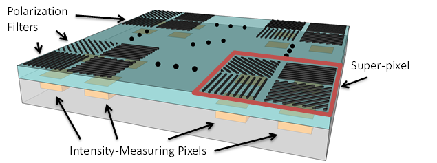
Figure 1: Division-of-focal-plane polarimeter sensor showing the repeating pattern of polarization filters grouped into super-pixels above an array of intensity-measuring pixels.
In general, we can model the behavior of each polarization
pixel as the composition of the pixelÆs conversion function acting on the
intensity of the light passed by the polarization filter. Using Mueller
calculus, the light passed by the polarization filter is represented by the
Stokes vector ![]() Āas a function
of the Stokes vector of the incident light,
Āas a function
of the Stokes vector of the incident light, ![]() :
:
![]()
where
![]() Āis the
Āis the ![]() Āreal-valued Mueller
matrix that characterizes the filter [Goldstein11].
The intensity component of the filtered Stokes vector is then passed to the
conversion function of the underlying pixel, which we will assume is linear and
noiseless:
Āreal-valued Mueller
matrix that characterizes the filter [Goldstein11].
The intensity component of the filtered Stokes vector is then passed to the
conversion function of the underlying pixel, which we will assume is linear and
noiseless:
![]()
where
![]() Āis the digital
value measured by the pixel;
Āis the digital
value measured by the pixel; ![]() Āis
the conversion gain of the pixel, which converts the intensity to digital
values; and
Āis
the conversion gain of the pixel, which converts the intensity to digital
values; and ![]() Āis the dark
offset of the pixel. The dot product
Āis the dark
offset of the pixel. The dot product ![]() Āselects only
the intensity component of the Stokes vector. This model can be simplified
somewhat by noting that only the first row of the Mueller matrix is required
and we can combine the conversion gain into the dot product. Thus, we let
Āselects only
the intensity component of the Stokes vector. This model can be simplified
somewhat by noting that only the first row of the Mueller matrix is required
and we can combine the conversion gain into the dot product. Thus, we let
![]()
and the polarization pixel model becomes
![]()
The vector ![]() Āis known as
the pixelÆs analysis vector. Note that the model does not include temporal noise,
quantization noise, or saturation effectsŚthey are beyond the scope of this
work.
Āis known as
the pixelÆs analysis vector. Note that the model does not include temporal noise,
quantization noise, or saturation effectsŚthey are beyond the scope of this
work.
When considering a super-pixel of polarization pixels, we group the individual pixel responses into a vector so that
where
![]() Āis the
super-pixelÆs analysis matrix, which is constructed by stacking the analysis
vectors
Āis the
super-pixelÆs analysis matrix, which is constructed by stacking the analysis
vectors ![]() Āfor each
pixel
Āfor each
pixel ![]() Āin the
super-pixel. Note that this model assumes that the illumination is either uniform
over the super-pixel or that all of the pixels in a super-pixel are co-located;
this is what causes the IFOV reconstruction errors that are dealt with in
[Tyo09].
Āin the
super-pixel. Note that this model assumes that the illumination is either uniform
over the super-pixel or that all of the pixels in a super-pixel are co-located;
this is what causes the IFOV reconstruction errors that are dealt with in
[Tyo09].
In the ideal case, all of the polarization pixels would have
identical and perfect analysis vectors and dark offsets, ![]() Āand
Āand ![]() ,
respectively. Additionally, this would lead to all of the super-pixels having
identical and perfect analysis matrices,
,
respectively. Additionally, this would lead to all of the super-pixels having
identical and perfect analysis matrices, ![]() . As mentioned
previously, this is not typically the case and deviations from the ideal can introduce
significant reconstruction errors. In light of this, the purpose of DoFP
polarimeter calibration techniques is to transform the non-ideal
polarization-pixel responses into the ideal polarization-pixel response.
. As mentioned
previously, this is not typically the case and deviations from the ideal can introduce
significant reconstruction errors. In light of this, the purpose of DoFP
polarimeter calibration techniques is to transform the non-ideal
polarization-pixel responses into the ideal polarization-pixel response.
In general, calibration techniques consist of a calibration function that takes a single pixelÆs intensity measurement or super-pixelÆs intensity measurement vector and returns an approximation of the ideal intensity value or vector that the pixel should have measured:
![]()
![]()
The ideal intensity value or vector comes from the same model, but with some ideal value for the analysis vectors and zero dark offsets.
The scalar, or ōgain and offset,ö calibration method presented in [York11] arises when each pixel is considered independently. Since we are trying to transform the linear polarization pixel response into the similarly linear ideal pixel response, we use a linear transformation as the calibration function:
![]()
The
parameters ![]() Āand
Āand ![]() Āare the
calibration gain and calibration dark value, respectively, and are determined
such that they minimize the squared L2, or Euclidian, distance between
Āare the
calibration gain and calibration dark value, respectively, and are determined
such that they minimize the squared L2, or Euclidian, distance between ![]() Āand
Āand ![]() :
:
![]()
![]()
Completing
the minimization by setting the partial derivatives with respect to ![]() Āand
Āand ![]() Āequal to zero
and solving the system of equations yields
Āequal to zero
and solving the system of equations yields
![]()
By
letting ![]() Āthis
simplifies to
Āthis
simplifies to
![]()
Unfortunately, the presence of ![]() Āin the
expression for
Āin the
expression for ![]() Āmeans that
the optimal calibration gain depends on the light we are trying to measure. This
is clearly unacceptable since we cannot accurately measure the light without an
appropriate value for both
Āmeans that
the optimal calibration gain depends on the light we are trying to measure. This
is clearly unacceptable since we cannot accurately measure the light without an
appropriate value for both ![]() Āand
Āand ![]() .
.
One solution to this problem is to make the approximation
that ![]() Āis a scalar
multiple of
Āis a scalar
multiple of ![]() . Then
. Then ![]() Āis approximately
constant and we can simplify
Āis approximately
constant and we can simplify ![]() Āto the ratio
of the length of
Āto the ratio
of the length of ![]() Āto that of
Āto that of ![]() :
:
This is equivalent to the expressions given in equations 7, 8, and 9 of [York11] if we take the ideal response as that of the best-performing pixel of the super-pixel rotated to match the orientation of the current pixel.
When we consider each super-pixel as a whole, we can derive the calibration function presented in [Myhre12]. This calibration function is similar to the scalar version, but the calibration dark value is expanded to a vector, and the calibration gains are a square matrix:
![]()
Again,
![]() Āand
Āand ![]() Āare
determined such that they minimize the squared L2 distance between
Āare
determined such that they minimize the squared L2 distance between ![]() Āand
Āand ![]() :
:
![]()
![]()
Completing this minimization by setting the partial derivatives equal to zero and solving the resulting system of equations leads to
![]()
in
the case where ![]() Āis square and
full rank or
Āis square and
full rank or
![]()
otherwise.
While these results are very similar to the scalar case, this calibration
function is clearly more general and powerful as it does not include ![]() Āin the expressions
for
Āin the expressions
for ![]() Āor
Āor ![]() Āand it makes
no further assumptions about the polarization pixels.
Āand it makes
no further assumptions about the polarization pixels.
The polarization pixel model ![]() Ācan be
interpreted as projecting the
Ācan be
interpreted as projecting the ![]() Āvector onto
the
Āvector onto
the ![]() Āvector and
applying some offset. Applying the scalar calibration function results in a new
projection
Āvector and
applying some offset. Applying the scalar calibration function results in a new
projection
where we have removed the offset and rescaled the analysis vector to the length of the ideal analysis vector. Thus the accuracy of this method depends on the actual and ideal analysis vectors pointing in the same direction.
Alternatively, the matrix calibration function multiplies each of the analysis vectors by a matrix:
![]()
As long as the analysis matrix has high enough rank, the gain matrix will be able to both scale and rotate the individual analysis vectors to match the ideal case. Because of this ability to rotate the analysis vectors, the matrix calibration technique should achieve significantly lower error rates than the scalar technique.
The two calibration functions were tested on a 300x300 pixel sub-region of the linear DoFP polarimeter described in [Gruev10]. This polarimeter is composed of linear pixels aligned with a repeating pattern of 2x2 blocks of linear polarization filters oriented at 0░, 45░, 90░, and 135░. Because it only has linear polarization filters and no circular polarization filters, the last component of its pixelsÆ analysis vectors is always zero, and it can only reconstruct the first three parameters of the Stokes vector.
Performing the evaluation requires two steps. The first is
to determine the analysis vectors for each pixel. Since the pixel model is
linear, we can simply measure the pixel responses under a variety of
illuminations and use a multivariate linear regression to solve for ![]() Āand
Āand ![]() Āfor each
pixel. The second step is to then calculate the appropriate calibration
parameters for each function and evaluate their performance. The apparatus used
to illuminate the polarimeter is shown in figure 2. By varying the adjustable
shutter, the intensity of the illumination,
Āfor each
pixel. The second step is to then calculate the appropriate calibration
parameters for each function and evaluate their performance. The apparatus used
to illuminate the polarimeter is shown in figure 2. By varying the adjustable
shutter, the intensity of the illumination, ![]() Ācan be
controlled. Varying the angle of the linear polarizer,
Ācan be
controlled. Varying the angle of the linear polarizer, ![]() , allows us to
generate values for
, allows us to
generate values for ![]() Āand
Āand ![]() Āon a circle
with a radius of
Āon a circle
with a radius of ![]() . The
calibrated photodiode lets us measure the absolute level of
. The
calibrated photodiode lets us measure the absolute level of ![]() . This
apparatus leaves the last value of the Stokes vector,
. This
apparatus leaves the last value of the Stokes vector, ![]() , at zero, but
since the polarimeter we are evaluating cannot measure
, at zero, but
since the polarimeter we are evaluating cannot measure ![]() Āit is
inconsequential.
Āit is
inconsequential.
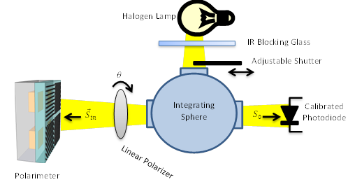
Figure 2: Apparatus for evaluating the calibration functions. It generates
uniform illumination with arbitrary values of ![]() , and
, and ![]() ,
, ![]() Āon a circle
of radius
Āon a circle
of radius ![]() .
.
The 300x300 pixel window was illuminated with 6 different
intensities of light, ranging from 2.5% to 100% of the dynamic range of the
polarimeter; and 9 different angles, equally spaced around the ![]() Ācircle. One
hundred samples were taken at each intensity-angle pair to reduce the effects
of temporal noise on the regression. This results in 5,400 samples taken for
each of the 90,000 pixels. Each pixelÆs analysis vector and dark offset were
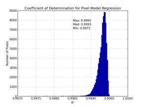
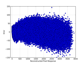
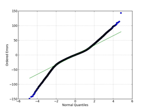
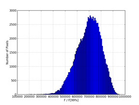
solved for using a basic multilinear regression. The histogram in figure 3 (a)
summarizes the coefficents of determination,
Ācircle. One
hundred samples were taken at each intensity-angle pair to reduce the effects
of temporal noise on the regression. This results in 5,400 samples taken for
each of the 90,000 pixels. Each pixelÆs analysis vector and dark offset were
solved for using a basic multilinear regression. The histogram in figure 3 (a)
summarizes the coefficents of determination, ![]() Āvalues, for
all of the regressions, which shows that the regressions are not perfect, but
do explain at least 99.7% of the variation in the sample data. Plot (b) shows
the reconstruction errors versus the predicted values, which has a slight
trend, but not significant compared to the range of the data. Plot (c) shows a
normal quantile-quantile plot of the errorsŚthis indicates that the error
distribution has longer tails than the normal distribution, but is otherwise
closely approximated by it. Finally, plot (d) shows a histogram of the ratio of
each regressionÆs F-value to the 99% significance F-value, all of which are
much greater than 1, which indicates that all of the regressions are
significant.
Āvalues, for
all of the regressions, which shows that the regressions are not perfect, but
do explain at least 99.7% of the variation in the sample data. Plot (b) shows
the reconstruction errors versus the predicted values, which has a slight
trend, but not significant compared to the range of the data. Plot (c) shows a
normal quantile-quantile plot of the errorsŚthis indicates that the error
distribution has longer tails than the normal distribution, but is otherwise
closely approximated by it. Finally, plot (d) shows a histogram of the ratio of
each regressionÆs F-value to the 99% significance F-value, all of which are
much greater than 1, which indicates that all of the regressions are
significant.
(a)ĀĀĀĀĀĀĀĀĀĀĀĀĀĀĀĀĀĀĀĀĀĀĀĀĀĀĀĀĀĀĀĀĀĀĀĀĀĀĀĀĀĀĀĀĀĀĀĀĀĀĀĀĀĀĀĀĀĀĀĀĀĀĀĀĀĀĀĀĀĀĀĀĀĀĀĀĀĀĀĀĀĀĀĀĀĀĀĀĀĀĀĀĀĀĀĀĀĀĀĀĀĀ (b)
(c)ĀĀĀĀĀĀĀĀĀĀĀĀĀĀĀĀĀĀĀĀĀĀĀĀĀĀĀĀĀĀĀĀĀĀĀĀĀĀĀĀĀĀĀĀĀĀĀĀĀĀĀĀĀĀĀĀĀĀĀĀĀĀĀĀĀĀĀĀĀĀĀĀĀĀĀĀĀĀĀĀĀĀĀĀĀĀĀĀĀĀĀĀĀĀĀĀĀĀĀĀĀĀĀ (d)
Figure 3: Statistics of the pixel model regression: (a) coefficients of determination, ![]() ; (b) reconstruction error vs. reconstructed pixel response; (c) normal quantile-quantile
plot; and (d) F-tests.
; (b) reconstruction error vs. reconstructed pixel response; (c) normal quantile-quantile
plot; and (d) F-tests.
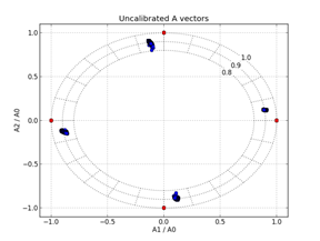
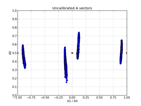
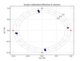
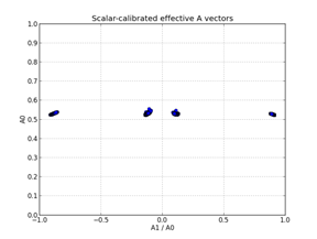
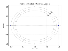
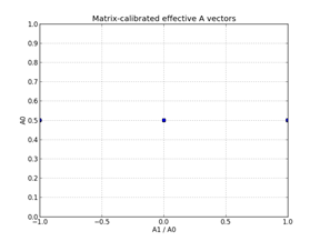
Both scalar and matrix gains were computed from the analysis vectors solved for with the linear regression. Figure 4 shows plots of the pixels analysis vectors and the effects of applying the calibration functions to the analysis vectors. Plots (a) and (b) show the actual analysis vectors of the pixels. They have a clear error relative to the ideal but little spread in the normalized A1-A2 space shown in (a), but very large spread in the A0 dimension. Applying the scalar gains results in plots (c) and (d). As expected, there is no change in the normalized A1-A2 space, but the variation in A0 is reduced dramatically. Finally, multiplying the vectors by their respective matrix gains results in plots (e) and (f). Since this calibration function is powerful enough to meet the ideal without any extra assumptions, the effective analysis vectors are transformed completely to their ideal values.
(a)ĀĀĀĀĀĀĀĀĀĀĀĀĀĀĀĀĀĀĀĀĀĀĀĀĀĀĀĀĀĀĀĀĀĀĀĀĀĀĀĀĀĀĀĀĀĀĀĀĀĀĀĀĀĀĀĀĀĀĀĀĀĀĀĀĀĀĀĀĀĀĀĀĀĀĀĀĀĀĀĀĀĀĀĀĀĀĀĀĀĀ (b)
(c)ĀĀĀĀĀĀĀĀĀĀĀĀĀĀĀĀĀĀĀĀĀĀĀĀĀĀĀĀĀĀĀĀĀĀĀĀĀĀĀĀĀĀĀĀĀĀĀĀĀĀĀĀĀĀĀĀĀĀĀĀĀĀĀĀĀĀĀĀĀĀĀĀĀĀĀĀĀĀĀĀĀĀĀĀĀĀĀĀĀĀĀ (d)
(e)ĀĀĀĀĀĀĀĀĀĀĀĀĀĀĀĀĀĀĀĀĀĀĀĀĀĀĀĀĀĀĀĀĀĀĀĀĀĀĀĀĀĀĀĀĀĀĀĀĀĀĀĀĀĀĀĀĀĀĀĀĀĀĀĀĀĀĀĀĀĀĀĀĀĀĀĀĀĀĀĀĀĀĀĀĀĀĀĀĀĀĀ (f)
Figure 4: Plots of the effective analysis vectors after calibration. Plots (a) and (b) show the pixelsÆ actual analysis vectors, (c) and (d) show the effect of applying scalar-calibration, and (e) and (f) show the effect of applying matrix-calibration. Plots (a), (c), and (e) show the vectors in the A1-A2 space, normalized by A0. The radius in these plots indicates how well the filters discriminate different polarizations of light. Plots (b), (d), and (f) have the same x-axis, but show A0 on the y-axis. These plots indicate the overall transmission ratio of the filters. In all plots the ideal values are indicated by red squares.
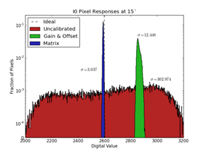
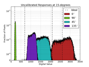
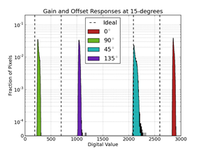
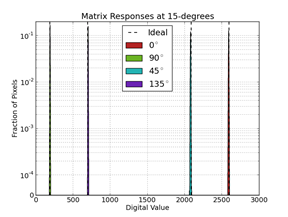
Figure 5 examines the results of applying the calibration
functions to the actual pixel responses. Histogram (a) compares all of the
super-pixelsÆ ![]() Ācomponents
uncalibrated response and the results of scalar and matrix calibrations with
the ideal response. The uncalibrated response has a very large spread, which
shows the non-uniformity of the filtersÆ analysis vectors. Applying scalar
calibration reduces this spread significantly, which indicates that the
non-uniformity is predominantly in the
Ācomponents
uncalibrated response and the results of scalar and matrix calibrations with
the ideal response. The uncalibrated response has a very large spread, which
shows the non-uniformity of the filtersÆ analysis vectors. Applying scalar
calibration reduces this spread significantly, which indicates that the
non-uniformity is predominantly in the ![]() ĀĀcoefficients
of the filters, but does not center the responses about the ideal value.
Finally, the matrix calibration further reduces the spread and centers the
responses about the ideal, which indicates that the matrix calibration function
accounts for significantly more of the non-uniformities and non-idealities in
the pixel responses. This agrees with the conclusions drawn from figure 4. Histograms
(b), (c), and (d) respectively show the uncalibrated, scalar-calibrated, and
matrix-calibrated responses of all of the polarization pixels when illuminated
with Āuniform linearly polarized light at
ĀĀcoefficients
of the filters, but does not center the responses about the ideal value.
Finally, the matrix calibration further reduces the spread and centers the
responses about the ideal, which indicates that the matrix calibration function
accounts for significantly more of the non-uniformities and non-idealities in
the pixel responses. This agrees with the conclusions drawn from figure 4. Histograms
(b), (c), and (d) respectively show the uncalibrated, scalar-calibrated, and
matrix-calibrated responses of all of the polarization pixels when illuminated
with Āuniform linearly polarized light at ![]() . In histogram
(b), it is clear that the spread of the responses is heavily dependent on the response
level. This is further evidence that the majority of the non-uniformities of
the filters is in the
. In histogram
(b), it is clear that the spread of the responses is heavily dependent on the response
level. This is further evidence that the majority of the non-uniformities of
the filters is in the ![]() Ācoefficients.
Further support for this is seen in the lack of this dependence in the
scalar-calibrated responses, which predominantly corrects
Ācoefficients.
Further support for this is seen in the lack of this dependence in the
scalar-calibrated responses, which predominantly corrects ![]() .
.
(a)ĀĀĀĀĀĀĀĀĀĀĀĀĀĀĀĀĀĀĀĀĀĀĀĀĀĀĀĀĀĀĀĀĀĀĀĀĀĀĀĀĀĀĀĀĀĀĀĀĀĀĀĀĀĀĀĀĀĀĀĀĀĀĀĀĀĀĀĀĀĀĀĀĀĀĀĀĀĀĀĀĀĀĀĀĀĀĀĀĀĀĀĀĀĀ (b)
(c)ĀĀĀĀĀĀĀĀĀĀĀĀĀĀĀĀĀĀĀĀĀĀĀĀĀĀĀĀĀĀĀĀĀĀĀĀĀĀĀĀĀĀĀĀĀĀĀĀĀĀĀĀĀĀĀĀĀĀĀĀĀĀĀĀĀĀĀĀĀĀĀĀĀĀĀĀĀĀĀĀĀĀĀĀĀĀĀĀĀĀĀĀĀĀĀĀĀĀ (d)
Figure 5: Histograms of linear polarization pixel responses when un-calibrated (a) and (b), scalar-calibrated (a) and (c), and matrix-calibrated (a) and (d) compared to the ideal response.
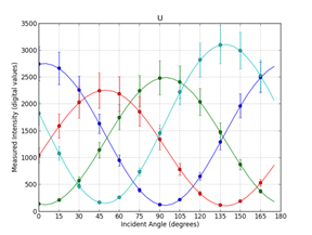
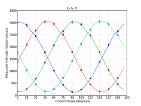
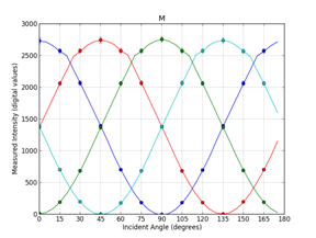
Finally, figure 6 shows the mean and standard deviation of
the un-calibrated, scalar-calibrated, and matrix-calibrated responses to
linearly polarized light as the ![]() Āand
Āand ![]() Ācomponents of
the incident light are swept about the circle with radius
Ācomponents of
the incident light are swept about the circle with radius ![]() . The plots of
figure 6 support all of the conclusions drawn from the histograms of figure 5
as the incident angle of polarization changes. We can see that as the incident
angle changes, the un-calibrated mean responses of the different orientations
of polarization pixels have a sinusoidal response, but have non-uniform
amplitudes and offsets. Both the scalar- and the matrix-calibrated data correct
a majority of this non-uniformity, however it is worth noting that there is a
significant offset from zero in the scalar-calibrated responses, and that the
peaks of the scalar-calibrated curves are not centered on the appropriate
angles. The matrix-calibrated responses clearly corrects for both problems.
. The plots of
figure 6 support all of the conclusions drawn from the histograms of figure 5
as the incident angle of polarization changes. We can see that as the incident
angle changes, the un-calibrated mean responses of the different orientations
of polarization pixels have a sinusoidal response, but have non-uniform
amplitudes and offsets. Both the scalar- and the matrix-calibrated data correct
a majority of this non-uniformity, however it is worth noting that there is a
significant offset from zero in the scalar-calibrated responses, and that the
peaks of the scalar-calibrated curves are not centered on the appropriate
angles. The matrix-calibrated responses clearly corrects for both problems.
(a)ĀĀĀĀĀĀĀĀĀĀĀĀĀĀĀĀĀĀĀĀĀĀĀĀĀĀĀĀĀĀĀĀĀĀĀĀĀĀĀĀĀĀĀĀĀĀĀĀĀĀĀĀĀĀĀĀĀĀĀĀĀĀĀĀĀĀĀĀĀĀĀĀĀĀĀĀĀĀĀĀĀĀĀĀĀĀĀĀĀĀĀĀĀĀ (b)
(c)
Figure 6: Mean and standard deviations of un-calibrated (a), scalar-calibrated (b), and matrix-calibrated (c) polarization pixel responses with varying incident angle of polarization.
We have shown two DoFP polarimeter calibration functions, one based on treating each pixel individually, and the other treating each super-pixel as a whole. Both were derived from a linear, noiseless model for a polarization pixel and were evaluated on an existing DoFP polarimeter. The parameters of the linear model were learned for each pixel of the polarimeter with very high confidence by performing a linear regression over 5,400 test images. The results show that while the scalar calibration technique reduces the reconstruction error greatly, it is not as effective as the matrix-based technique. This was predicted from the derivation of the two methods as the scalar calibration function required making extra assumptions about the nature of the pixels, which were unnecessary in the matrix case.
DoFP: Division of Focal Plane
DoT: Division of Time
DoA: Division of Amplitude
IFoV: Instantaneous Field of View
In order of importance:
[York11] York, T; Gruev, V; ōCalibration method for division of focal plane polarimeters in the optical and near-infrared regime,ö SPIE Proceedings, 2011, http://dx.doi.org/10.1117/12.883950
[Myhre12] Myhre, G; Hsu, W-L; Peinado, A; Pau, S; ōLiquid crystal polymer full-stokes division of focal plane polarimeter,ö Optics Express, 2012, 27393-27409, http://dx.doi.org/10.1364/OE.20.027393
[Gruev10] Gruev, V; Perkins, R; York, T; ōCCD polarization imaging sensor with aluminum nanowire optical filters,ö Optics Express, 2010, 19087-19094, http://dx.doi.org/10.1364/OE.18.019087
[Goldstein11] Goldstein, D; ōPolarized Light,ö CRC Press, 2011
[Tyo09] Tyo, J; LaCasse, C; Ratliff, B; ōTotal elimination of sampling errors in polarization imagery obtained with integrated microgrid polarimeters,öOptics Letters, 2009, 3187-3189, http://dx.doi.org/10.1364/OL.34.003187
[Gao11] Gao, S; Gruev, V; ōBilinear and bicubic interpolation methods for division of focal plane polarimeters,ö Optics Express, 2011, 26161-26173, http://dx.doi.org/10.1364/OE.19.026161
[Shwartz06] Shwartz, S; Namer, E; Schechner, Y; ōBlind Haze Separation,öĀ IEEE Computer Society Conference on Computer Vision and Pattern Recognition, 2006, 1984-1991, http://dx.doi.org/10.1109/CVPR.2006.71
[Tyo06] Tyo, J; Goldstein, D; Chenault, D; Shaw, J; ōReview of passive imaging polarimetry for remote sensing applications,ö Applied Optics, 2006, 5453-5469, http://dx.doi.org/10.1364/AO.45.005453
[Cronin03] Cronin, T; Shashar, N; Caldwell,R; Marshall, J; ōPolarization Vision and Its Role in Biological Signaling,ö Integrative and Comparative Biology, 2003, 549-558, http://dx.doi.org/10.1093/icb/43.4.549
[Goldstein06] Goldstein, D; ōPolarization properties of Scarabaeidae,ö Applied Optics, 2006, 7944-7950, http://dx.doi.org/10.1364/AO.45.007944