ESE297 - Intro to Undergraduate Research
From ESE497 Wiki

ESE297 - Introduction to Undergraduate Research was created for students who wish to do Undergraduate Research projects in Robotic Sensing under Professor Nehorai, the ESE Department Chair. This course is offered as ESE297 for 2 credits and is typically offered in the spring and summer. Students will learn how to implement sensor array signal processing algorithms on the LabVIEW for Robotics Starter Kit robots shown above using both Matlab and LabVIEW and develop Brain Computer Interface (BCI) algorithms using EEG signals. Students can then apply this knowledge to individual research projects in Robotic Sensing in subsequent semesters. ESE297 does not qualify as an EE electvie.
Logistics
- Meeting Time: Tues-Thursday, 1-4 pm in Bryan 316 from 5/24 - 7/16
- Holidays: 5/28, 7/4
- Instructor: Ed Richter
- Syllabus
- Expectations: The work load is estimated to be 10 hours/week. In the summer, the expectation is 20 hours/week. That is, students who earn an A will spend many unsupervised hours outside of the class meeting times. Grading is based on your Homework and your Projects. Late work will be accepted with a penalty. Please see the syllabus for due dates.
Lecture Notes
- Topic 1: Acoustic Source Location Background and Theory (Slides 1-19)
- Additional references:
- Homework 1: Read the material that we discussed in our meeting today and the additional references listed above.
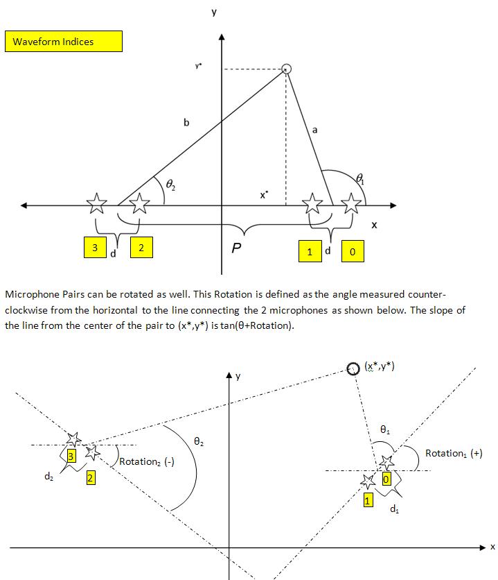
- Homework 2: Using this figure, derive the general equations for the source location (x*,y*) which include the rotation of both pair, i.e., the intersection of the 2 lines. Verify that the formula on slide 10 of the lecture notes is correct for the special case where
- y1 = y2 = 0
- Rotation1 and Rotion2 = 0
- X1=P/2
- X2 = -P/2
- Topic 2: Data Acquisition Basics
- LabVIEW Tutorial
- Code up examples in LabVIEW for slides 11, 14, 27, 31, 36, 38, 41. Put each one in a separate VI and demo to me or T/A.
- Configure LabVIEW options as shown in slides 15-17
- Exercises 1,2,3
- Homework 3 - Finish Exercises
- Assign Project1 - Simulation
- Homework 4 - Finish ComputeAngle.vi (in Project1 -> RoboticSensing.zip -> micSourceLocator.lvproj -> My Computer -> ComputeAngle.vi) and ComputeIntersection.vi
- Additional Resources
- Conditionally append values to an array in a loop
- How to Create and Array on the Front Panel
- LabVIEW tutorial, LabVIEW 101
- Data Acquisition Basics
- Homework 5 - Finish exercise
- Homework 6 - Connect wires from A00 and AO1 to AI0+ and AI1+ (remove wire from Banana A to AI0+). Make sure that the Prototyping Power is on. Modify your vi from Homework 5 to collect samples from both AI0 and AI1. Then open DelayedChirp2DAC.vi and run this vi. You shouldn't modifiy DelayedChirp2Dac.vi. Run your modified Homework 5 vi and zoom in in the time and frequency domain to examine the waveforms in detail. Describe in detail what you see. Measure the difference in time between both channels. Hint: Start and stop your Data Acquisition vi until the entire signal is in the middle of the buffer.
- LabVIEW Tutorial
- Topic 3: Signal Processing Basics
- Cross Correlation
- Homework 7
- Plot the Cross Correlation of the 2 channels from Homework 6 and see if the peak is shifted from the middle, the number of samples you measured from the previous step.
- Hints:
- Functions -> Express -> Signal Analysis -> Conv & Corr -> Cross Correlation
- This function requires that you extract the 2 channels from the DDT. To do this, use Functions -> Express -> Sig Manip -> From DDT -> Single Waveform -> Channel 0 and then again for Channel 1. Connect the outputs of these to the X and Y inputs.
- Before you plot the Cross Correlation, extract the 1D array of scalars using the From DDT so that the X-Axis is in samples.
- Look at the help on the Cross Correlation for details.
- Hints:
- Plot the Spectrogram of Channel 0.
- Hint: There is a good Spectrogram example that ships with LabVIEW. Go to Help -> Find Examples... and search for STFT -> STFT Spectrogram Demo.vi. You can copy from this example and paste it into your code.
- Plot the Cross Correlation of the 2 channels from Homework 6 and see if the peak is shifted from the middle, the number of samples you measured from the previous step.
- Homework 7
- Tutorial
- Homework 8- Finish exercise from tutorial.
- Homework 9- Use the Signal Processing Palette in LabVIEW to generate 2 sinusoid waveforms (Signal Processing -> Waveform Generation -> Sine Waveform) with two different frequencies. Add these together and implement 2 separate filters for this signal (Functions -> Express -> Signal Analysis -> Filter) to extract the original sinusoids. Plot these outputs in the time domain. Also, plot them in the frequency domain (Express-> Signal Analysis -> Spectral). Make sure you can identify the frequencies corresponding to the input sinusoids in the frequency domain. Next, add (as in addition) Gaussian White Noise to the sum of the 2 sinusoids (Signal Processing -> Waveform Generation -> Gaussian White noise). Plot the spectrum of the unfiltered signal and identify the frequencies corresponding to signal and noise again. Increase the standard deveiation of the WGN and modify your filter to improve the quality of the filtered signal. Also, looking at the sum of the 2 sinusoids and the noise, what is the relationship between the Standard Deviation of the WGN and the amplitude of the noise. Plotting the histogram of the noise (Express -> Signal Analysis -> Histogram) might help? Note: If your graph X-axis is in absolute time instead of seconds, right click on the graph and select Properties -> Display Format -> X-Axis and set it to SI units.
- DSP Lecture by Dr. Jim Hahn (for reference)
- DSP Configurations Lecture by Dr. Jim Hahn (for reference)
- Cross Correlation
- Topic 4: Brain Computer Interface (BCI)
- Performing an Offline Analysis of EEG Data using BCI2000
- BCI2000 is installed at c:\BCI2000. The tools and data folders referenced in the tutorial are at c:\BCI2000\tools and c:\BCI2000\data
- To launch BCIViewer, browse to tools\BCI2000Viewer and double click on BCI2000Viewer.exe. Pay particularly close attention to States StimulusBegin and StimulusCode.
- To launch OfflineAnalysis, browse to tools\OfflineAnalysis and double click on OfflineAnalysis.bat
- Introduction to Signal Detection/Classification
- How to collect EEG data using BCI2000 and the Emotiv headset
- Introduction to EEG Physiology (reference)
- Performing an Offline Analysis of EEG Data using BCI2000
Projects
- Project1: Implement algorithm using microphone array
- Project2:_Triangulation_with_sbRIO_robots
- BCI Projects
- Project3: BCI Offline Analysis - Signal Detection
- Plot R^2 for all Channels/Frequency Pairs
- Analyzing BCI2000 dat Files
- Start with OfflineAnalysisSpectral.m. This is the file you will modify for this project.
- Open in Matlab. Click on File-Set Path and "Add with subfolders" the Tools folder from the BCI2000 folder
- Click the Run arrow. Select eeg1_1.dat, eeg1_2.dat and eeg1_3.dat. Click Open
- Remove the DC (average) for all 64 channels
   for ch=1:size(signal, 2)
       signal(:, ch)=signal(:, ch)-mean(signal(:, ch));
   end
- Implement CAR Spatial Filtering using the BCI2000 funtion carFile
signal = carFilt(signal,2) ;
- For every channel compute the power spectrum for every segment of 80 samples every 40 samples for both condition==0 and condition==2 and average them. Create two 3D array of PowerSpectra of size(NumFrequencies,NumChannels,NumTrials) for both conditions.
- Compute the R^2 function for all Channel/Frequency pairs
- Plot the R^2 values for all Channel/Frequency pairs using the BCI2000 function calc_rsqu. It should look similar but not identical to the graph on the tutorial.
- Useful Matlab Functions:
- find
- spectrogram
- surf
- Project4: BCI Offline Analysis - Signal Classification
- Combine best Channel/Frequency pairs using eeg1 (use lda.m)
- Collect your own data using the Emotiv Headset
- Combine best Channel/Frequency pairs using your own data
- Plot the power in the 4 best Channel/Frequency pairs for the action and the rest conditions using the eeg1 data vs. trial
- Plot the action and rest results of the LDA vs. trial
- Plot the ROC for the 4 best Channel/Frequency pairs and the LDA
- Results
- Useful Matlab Functions:
- subplot
- save, load
- squeeze
- Project 5: Move sbRIO robots based on BCI algorithm using EEG1 data
- Re-Package your Matlab code into 2 functions that
- 1) Read the trials from the .dat files and return 1 trial every time it is called.
- 3) Computes the LDA measure from the current trial.
- Test these new functions in a for loop in Matlab and make sure you LDA results match the results from before
- Call your matlab functions from inside BCI.vi and move the robots every time the action is detected. Verify that you get the number of errors you expected and that the LDA calculation matches from before.
- Re-Package your Matlab code into 2 functions that
- Project 6: Implement in real-time with Emotive headset