Electric Longboard

Project Overview

When riding a Longboard for commuting or exercise, there is no way to know exactly how far or how fast one has ridden. Our goal for this project was to modify the Longboard riding experience by enabling someone to measure and record data about their ride. Using a GPS chip and an encoder on the wheel we programmed a Raspberry Pi 2 Model B to collect data from the board. We could then display the data on a map of the area tracing the route taken. This design enhances the Longboard riding experience by making it interactive and goal driven while also yielding tangible results.

Team Members

• Max Cetta
• Jacob Frank
• Alden Welsch (TA)

Objectives

1. Use GPS data to track distance and location of rides
   1. Use the serial port to connect to the GPS.
   2. Read data and write it into a text file.
   3. Display data
2. Have an encoder on the wheel to measure top ground speed and average speed over a ride
   1. Designing and printing the encoder
   2. Wiring the ADC and using SPI pins to communicate with the Raspberry Pi
   3. Writing code to filter and interpret the data to locate peaks

Challenges

1. Receiving data from the GPS chip
2. Interpreting the data
   • Isolating desired data from the GPS data stream which provided other information that was not useful for our project
3. Displaying the data
   • How to get the data off the Raspberry Pi
   • Displaying the riders position on a map
   • Displaying the riders velocity on computer screen
4. Designing Encoder
   • Ensuring mount would attach to the truck of the Longboard
   • Making sure the mounts were able to house the LED and photocell reliably and safely
   • Stabilizing results across all lighting conditions and riding surfaces
5. Hooking up the Analog to Digital Converter
   • Locating the SPI pins and correctly wiring them to the ADC
   • Building the voltage divider
   • Choosing the resistance to use for more rapid photocell saturation
6. Writing code to read the Encoder values, filter, and convert them to Kilometers per hour
   • Creating a properly sized filter to stabilize noise in data
   • Locating a peak in the data and ensuring that only 1 peak was counted
7. Environmental effects on GPS accuracy
   • Concrete, heavy clouds and other structures will obscure view to satellites
   • Locating and eliminating unreliable data
   • Substituting encoder data for these instances
8. Mounting
   • Taking all of our components and putting them in a compact container which can be secured to the longboard
   • Maintaining as light a design as possible considering the board is being manually powered
   • Keeping all the components safe and dry

Solutions

Receiving Data from the GPS

To receive data from the gps chip we looked at the data sheet for the baud rate, parity, stop bits, and byte size and declared them for the open serial port ttyAMA0. Opening the serial port required a series of terminal commands that disconnected the port from the raspberry pi so it could be hooked up to the GPS. For more info check out our How to page

def set_up_gps():
        ser = serial.Serial(
        port = '/dev/ttyAMA0',
        baudrate = 9600,
        parity = serial.PARITY_NONE,
        stopbits = serial.STOPBITS_ONE,
        bytesize = serial.EIGHTBITS,
        timeout=1
        )
     counter=0
     return ser

Interpreting The Data We Received

Below is an example of what the data we read from the serial port looked like:

$GPGSV,3,2,12,11,55,089,38,13,23,302,22,15,01,328,,17,34,230,25*78
$GPGSV,3,3,12,28,51,307,29,30,82,255,38,46,48,193,,51,42,206,*78
$GPGLL,3838.84048,N,09019.01465,W,220705.00,A,A*7E
$GPRMC,220706.00,A,3838.83954,N,09019.01492,W,3.123,189.68,250416,,,A*78
$GPVTG,189.68,T,,M,3.123,N,5.783,K,A*39
$GPGGA,220706.00,3838.83954,N,09019.01492,W,1,08,1.15,164.5,M,-32.0,M,,*64
$GPGSA,A,3,30,07,08,13,01,17,28,11,,,,,2.33,1.15,2.02*06

At first we didn't understand what these values were, but the GPS chip that we bought came with a data sheet that explained them. The values at the beginning of the lines are called message IDs. So to find velocity, for example, we had to look for the lines that started with $GPVTG which spits out values that correspond to course over ground speed. Lines with this message ID had 9 comma separated values that followed it (sometimes some of these values were blank, as in the example above). The value that corresponded to kilometers per hour was the value 7 down from $GPVTG: In the example above the rider was going 5.783 kilometers per hour. A similar process was used to find Longitude and Latitude.

Displaying the Data

Velocity

 speeds=[] #initialize array to store speeds
 ser=set_up_gps() #set_up_gps() connects to and returns values from the serial port. These values are stored in ser
 x=ser.readline() #readline() reads a line from the serial port and we store this value in x
             
 save_gps_to_file(x) 
             
 array=x.split(',') #the split function stores the values from each line in an array. *See below for more detailed description*
             
 if(array[0]=='$GPVTG'):
      if(array[7]!= ''):
          current_speed=array[7] #stores the value in array[7], which is kilometers per hour, in current speed
          print current_speed
          speeds.append(float(current_speed)) #Current_speed is a string so we need to convert it to a float. 
                                              #Then we add the value of the current speed to our speeds array.
          
          max_speed=max(speeds)  #every time we add a value to the speeds array we use the max function 
                                 #for arrays which returns the largest value in the array. We store this value in variable max_speed 

          total_speeds=0
          for x in speeds: #we iterate through all the values in speeds and add them up to get total speed
              total_speeds=x+total_speeds
          average=total_speeds/len(speeds) #to get average speed we divide total_speeds by the amount of speeds recorded

We wanted to display the riders current velocity during the ride and at the end of the ride display their max speed and average speed. To display the data the rider's velocity, we had to use pythons split() method for strings. The split method takes in a string as a parameter:let's call this string parameter the separator. When you call the split method on a string it separates the string by the separator you input as its parameter and the method returns an array with every element between the separators in the string stored in a different index in the array.So, In our program, we read a line from the serial port and stored it in a string x. Then we called x.split(",") which stored each line we read as an array with each value that was separated by a comma in a different index in the array. To find velocity we created an if stated that checked for the condition array[0]=="$GPVTG". Array[0] is what each line would start with--the message ID. Once this condition was met we knew that the 7th index in the array contained the rider's velocity in kilometers per hour. Every Time we read a velocity value we stored it in a variable current_speed and then printed it out. Then we stored this value in an array called speeds. At the end of the ride we called the max function (a built-in python function which returns the greatest value in an array) on speeds which returned the greatest value in our array--the rider's max speed--and printed it. To get the rider's average speed we iterated through speeds and added up all its values to get total_speeds and then then divided it by len(speeds) which returns the size of the array to get the rider's average speed and printed it.

Mapping

We also wanted to display the rider's route on a map. To do so we first had to save our GPS data to a text file. We did this by creating these methods:

def create_gps():
    filepath_GPS = '/media/pi/USB DISK/gps/GPS.txt'
    f=open(filepath_GPS,'w')
    f.write('starting...')
    f.write('\n\n')
    f.close()
    
    
def save_gps_to_file(x):
    filepath_GPS = '/media/pi/USB DISK/gps/GPS.txt'
    f=open(filepath_GPS,'a')
    f.write(x)
    f.write('\n\n')
    f.close()

Python's open method takes in two strings as parameters. The first is the name of a text file. The second is either a 'w' or a 'a' . The 'w' parameter tells the computer to create a new file with the name of the file listed in the first parameter; if a file with the same name already exists the computer will overwrite it. The open method by default will search for and create the file in the same folder that the python script is saved in. However, we wanted the file to be stored on our usb. To do so we had to direct it there. We did so by calling filepath_GPS = '/media/pi/USB DISK/gps/GPS.txt' .When the method is called with the "a" parameter, the computer checks for a file with the name given in the first parameter and if it exists, when f.write() is called, it appends to it. So, create_gps() creates the text file that we will later append to it by calling our save_gps_to_file(x) method. save_gps_to_file(x) takes in a parameter x, opens a text file for appending data and and writes whatever value is stored in x to it. After defining save_gps_to_file(x) we call it in the main method of our program. In the main method, x holds the data read from the GPS chip through the serial port.

Test Run

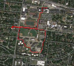
At the end of the ride the user can plug the USB drive into their computer and send the gps.txt to http://www.gpsvisualizer.com which displays where they went on a map. Below is an example of what this looks like using data we collected in one of our test rides:

Designing Encoder

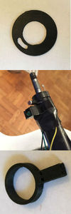
For the encoder first we started with a six slit disk for the wheel. When spun the wheel would revel the LED to the photocell 6 times a rotation. We also 3D printed simple blocks for the LED and photocell mounts that would have been glued to the truck. It quickly became apparent the simple box was not going to be sufficiently secure.

(Left) First iteration of six slitted disk. (Center) 3D printing six slitted disk design. (Right) First iteration of photocell mount.

(Top) First iteration of single slitted disk design. (Center) Final encoder mounts and spacers attached to the truck of the longboard and wired up. (Bottom) First iteration of the ring design for the photocell mount, meant to increase stability.

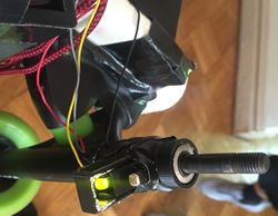
To solve the problem of security we added a ring to go around the truck with a box on top to house the LED and photocell respectively. Once on the truck we wanted to secure the spacing so we created specific mm spacers to go in between the wheel, photocell mount, and LED mount. After we started getting readings from the ADC we realized we only needed to measure single rotations as opposed to fractions of rotations and so we printed another ring with one larger hole to go around the wheel.

Shield designed to reflect LED light lined with aluminum foil.

Final shielded encoder design.

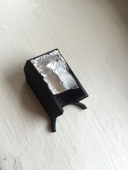
We were still not getting peaks with enough definition across surfaces and in different lighting conditions so we tried a number of filters that calculated standard deviations and means of data and tried to locate values that would cross a constantly updated filter, but none of these worked so we 3D printed another piece to act as a shield for the LED. This shield was lined with aluminum foil to reflect the LED light and once secured we finally got defined peaks over surfaces and in different lighting conditions.

Hooking up the Analog to Digital Converter

Hooking up the mcp3002 ADC required finding data sheets for the raspberry pi and the ADC in order to match the SPI pins and correctly wire the channel, voltage and ground. Once we had everything wired we could manipulate the circuit connected to channel 0. In order to read input from the ADC we needed to install spidev through the terminal and use it to open the SPI pins as explained in our How-to page. Initially we just had the photocell connected in series with a resistor to a voltage source, but our values we not highly responsive and made little sense. After a number of trials we discovered that we needed a voltage divider and connected one lead of the resistor to the ground. This way the photocell had a resistor pull-up that increases the saturation rate of the cell and gave us much more defined data from the ADC. Once this was all hooked up we could experiment with different resistor values based on the average ambient light we were experiencing and the subsequent average photocell resistance.

Reading ADC Values

Once we read ADC values we realized there was noise in the data. To correct this, we had to create a filter that used a rolling average. Below is the code we used to take ADC readings:

def reading():
    filter_size=12000
    filter=[0 for i in range(filter_size)]
    while(i<filter_size):
        x=read()
        filter[i]=x
        i=i+1
    total=0
    for reading in filter:
        total=total+reading
    return total/len(filter)

To decide on the filter size for the data we had to calculate how fast our max speed would require we read values. We thought 20 kph would be a fair max ground speed; based on this max speed, we divided by .95kph to get approximately 21 rotations per second. To record all these peaks we needed at least 3 times that many readings for the array to work. So multiplied by 3 was 63, then 1 divided by 63 was the time of the sample multiplied by 1.2 MHz yielded about 19,000 readings. Accounting for calculation time and just to be safe we brought the filter_size down to 12,000. Once we determined our filter_size, we repeatedly took readings from the ADC in our while loop and stored them in an array called filter. Once we had 12,000 readings we iterated through all the values in filter added them up and then returned their average to get our filtered ADC reading.

Writing code for the Encoder

After writing code to get filtered readings from the ADC we had to figure how we could detect a rotation for the skateboards wheel and then convert rotations to kilometers per hour. Here is the code for our encoder method, which returns the rider's speed:

def encoder():
    rotations=0
    queue=[0 for i in range(3)]
    while(i<3):
        queue[i]=reading()
        i=i+1
    previous_millis=0
    while(True):
             current_millis=millis()
             if((queue[1]>queue[0]) and (queue[1]>queue[2])):
                 rotations=rotations+1
             queue[0]=queue[1]
             queue[1]=queue[2]
             queue[2]=reading()
             if((current_millis-previous_millis)>1000):
                current_speed=rotations*.95
                print current_speed
                previous_millis=current_millis
                return current_speed

To detect a peak, we intialized an array called queue to hold three filtered readings. We took a filtered reading() and stored it in queue[0] then another filtered reading and stored it in queue[1] and a third reading that we stored in queue[2]. We then checked if(queue[1]>queue[0] and queue[1]>queue[2]). We set this condition because the reading in queue[1] would be greater than queue[0] and queue[2] if the readings for queue[0] and queue[2] occurred when the led was in line with the covered part of the disk and the reading for queue came in when the LED was in line with the slit in our disk. The value in queue[1] would be greatest because the photo cell returns greater values when exposed to more light. So, If this condition was met we could say the wheel had undergone a rotation so we incremented our rotations variable by one. Whether or not the condition in the if statement was met, meaning we had detected a rotation, we shifted the readings in our queue over: queue[0]=queue[1], queue[1]=queue[2] and then we took a new filtered reading() and stored it in queue[2] and checked the if statement again. When we first wrote the code for our encoder we would take three new reading()s every time and compare them. We realized, however, that we were missing peaks this way. We really needed to check every three consecutive readings to detect a peak. Reassigning the values in the queue solved this problem.

Now that we could count a rotation of the wheel we had to convert rotations to kilometers per hour. In order to do so we needed to be able to detect the time that occurred between a certain amount of rotations. To keep track of time we had to first import time at the beginning of our program. Python's time library includes a method time() which, when called, returns the amount of time that has elapsed since the program started running. We wanted to detect the milliseconds that had passed since so we created a method mills() that returned time.time()*1000--milliseconds elapsed since the start of the program. After creating this method we wanted to use it to check the size of the rotations variable every second. To do so we created a variable previous_millis which was initially set to zero and a variable current_millis which we set it equal mills() every time we took a new reading(). Every time, after checking for a rotation and then taking a new reading, we checked if((current_millis-previous_millis)>1000). If this condition was met it meant that a second had passed. When the program first runs current_millis will be roughly equal to zero because the program had just started. Every time we take new reading()s the value of current_millis grows because time continues to elapse since the program was ran. Eventually a second will pass and current_millis will be greater than 1000 (1000 milliseconds=1 second) so the condition in the if statement will be met. After we enter the if statement we set previous_millis=current_millis. We need to update previous_millis so we can check the value of rotations every second and not just the first second.

Now that we were able to check the size of rotations every second we needed to be able to convert rotations per second to kilometers per hour. To do we set current_speed=rotations*.95. We multiplied by .95 because the diameter of the wheel was 84 millimeters; 84 multiplied by pi is the circumference in mm, divided by 1,000,000 converts the circumference to kilometers. Assuming one rotation per second we multiply by 3,600 to convert to kilometers an hour, which is 0.95 kph per one rotation a second. Then we multiply by our sampled rotations per second to get speed. ((km/hr) / (rotations/second)) * (sampled rotations/second)

Environmental effects on GPS accuracy

Concrete, clouds and other environmental factors can block the GPS signal. When this happened we would not get any velocity values. We wanted to record the rider's velocity throughout the whole trip so when the gps chip was unable to receive reliable data we started storing the velocity values recorded by our encoder. To detect when we were not getting GPS values for velocity we had to search for the $GPVTG message Id as usual and then looked for the condition if(array[7]==" " ). If this condition was met, it meant we weren't getting velocity values because the index of the array where there should be a velocity value--array[7]--was blank. So, if the velocity value in array[7] was blank we ran encoder() and appended the value it returned to our speeds array that we were previously appending the values returned by GPS to.

Mounting

Mounting all of the components meant 3D printing a plate to hold the raspberry pi and an enclosure for the breadboard and wires. In addition holes for the GPS wires and a mount of the GPS on the outside of the cover were added. After the pi was secure we were able to solder the wires to the encoder on the wheel and attach them to the breadboard.

GPS

In order to track the path and distance traveled during a ride we needed a GPS chip to acquire coordinate and velocity data from satellites. Receiving this data required first opening the serial port, and then sending it through the serial port to the Raspberry Pi. A little bit of python code allowed us to readline() data at 1 Hz, which we could print to the serial monitor and write to text files we opened and appended. which would then save the data to a Text file. Once saved, we could parse the data, separated by commas, into an array and locate by array idex the coordinates and velocities we desired. We were able to display our data on a map of Washington University's campus using a website. In order to live stream our data from a remote source we then had to connect the Raspberry Pi to WiFi. Using an Edimax N150 we could configure the USB ports through the terminal allowing for consistent WIFi connectivity during a ride. Once this was done we could remote shell login and receive live data on our laptops.

Encoder

The encoder began as a matter of 3D printing. Making sure that the housings for the LED and photocell were secure and precisely spaced was an issue we faced through many iterations of the design. Once it was printed it became a matter of wiring and coding. Ensuring that the Encoder circuit worked reliably ended up being a matter of mechanics, circuitry, and programing. The Raspberry Pi does not take analog inputs through its GPIO pins so we had to use the mcp3002 Analog to Digital Converter to interpret analog signal from the photocell and convert them to readable values for the SPI pins. In addition to wiring the ADC we had to build a voltage divider that would give reliable values in light spaces and indicate ticks on the wheel with significant disparities. Once we had those values printing reliably and steadily we had to create a number of filters to average and interpret those values. By nesting while statements with filters and if statements we were able to create a counter that would count once for every time a stream of values went above a threshold. By putting that inside a delta time loop we could print the number of rotations per second. Finding that threshold was another matter entirely consisting of numerous trials with filter size and calculation rates. In the end by adjusting the value of the resistor in the voltage divider and creating a shield for the LED we were able to stabilize the values and locate a steady threshold.

Budget

Item	Quantity	Price	Vendor	Link
GPS Receiver - GP-20U7 (56 Channel)	1	$15.95	Sparkfun	https://www.sparkfun.com/products/13740
Mini Photocell	2	$1.50	Sparkfun	https://www.sparkfun.com/products/9088
Analog to Digital Converter - MCP3002	1	$2.30	Sparkfun	https://www.sparkfun.com/products/8636
Raspberry Pi 2 - Model B (8GB Bundle)	1	$49.95	Sparkfun	https://www.sparkfun.com/products/13724
Resistor Kit - 1/4W (500 total)	1	$7.95	Sparkfun	https://www.sparkfun.com/products/10969
LED - Basic Green 5mm	2	$0.35	Sparkfun	https://www.sparkfun.com/products/9592
Tontec® Raspberry Pi Case	1	$7.98	Amazon	http://www.amazon.com/Tontec%AE-Raspberry-Black-Enclosure-Transparent/dp/B00NUN98UW?ie=UTF8&psc=1&redirect=true&ref_=od_aui_detailpages00
KMASHI 10000mAh Battery	1	$13.99	Amazon	http://www.amazon.com/KMASHI-10000mAh-External-Battery-Portable/dp/B00JM59JPG?ie=UTF8&psc=1&redirect=true&ref_=oh_aui_detailpage_o04_s00
Total		$101.82

Gantt Chart

Timeline

Results

Encoder

Once we had our filters set and the code to locate peaks working with the shield over the LED the encoder worked very reliably. The only problem was when we were stopped we got extremely high numbers. To solve this we have started a filter to take out extraneous values when stopped. When stopped we received high counts in the hundreds so they are easy to filter out. We set the threshold as 20 kph seeing as that was our calculated maximum reliable speed.

GPS

The GPS ended up working essentially perfectly for our purposes, in addition to being supplemented by the encoder in times of low visibility. Concrete caused minor discrepancies, but ended up being less of an issue than originally anticipated.

WiFi

We got the WiFi dongle working with laptops, and had the data live streaming to them. Unfortunately we experienced tragedy during a test run and broke the WiFI dongle.

Gantt Chart and Timeline

At the beginning of the semester we thought we were going to be making a motorized electric longboard. After a month of searching for parts and trying to learn about motors and batteries we found out we were not going to be able to do it. At that point we changed our whole project outline to match a new vision going forward. We moved to the encoder and GPS idea, while also hoping to add headlights towards the end of the semester. We did not correctly anticipate the amount of time and energy simply setting up a development board, designing a part, importing libraries and making sure we had the correct hardware for connecting parts could take. After all the dirty work was done we were finally able to get to the interesting part of the project and were able to condense our timeline.