55.4.5 Displaying modal contribution factors

After the first plug-in has analyzed the data and written the results back to the output database, you can view the modal contribution factors. Start the second plug-in by selecting Plug-insNVHPlot modal Contribution Factors from the main menu bar in the Visualization module. The plug-in displays the Open ODB dialog box, and you enter the name of the output database from which to read. The plug-in then displays the Select Steps dialog box, as shown in Figure 55–2:

Figure 55–2 The Select Steps dialog box.

You must select the Valid Frequency Step and the Valid SSD Step from which you will generate plots. In addition, you must choose one of the following types of variables to plot:

Magnitude of MCF
Phase of MCF
Magnitude of sum
Phase of sum
Rank

The magnitude or the phase of the sum indicates the summation of modal contribution factors over all the modes. This is same as the ABAQUS output variable (POR, U, V, or A).

When you click Continue, the plug-in displays the Plot MCF dialog box. Click the Frequency Step/SSD Step button to select different frequency and steady-state dynamic step.

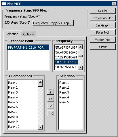
Click the Selection tab to select the following:

The response point.
The frequency of interest, if you are plotting a bar graph, a polar plot, or a vector plot.
Any number of Y components to plot. You add a Y component by clicking >; you remove a Y component by clicking <. You can add or remove all of the Y components by clicking the >> or << buttons respectively.

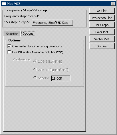
The Selection tabbed page is shown in Figure 55–3:

Figure 55–3 The Selection tabbed page.

Click the Options tab to select the general plot options. In addition, if you select POR-based results, you can select the P Reference value for XY and projection plots. From the buttons on the right side of the Plot MCF dialog box, select the type of plot to create.

Click XY Plot to generate the spectrum for the magnitude or phase of MCF. For mode-ranking selection, the plug-in creates X–Y plots for the modes corresponding to the specified ranks.
Click Projection Plot to plot the projection of the selected MCF onto the corresponding total sound pressure level across the spectrum. You can use this plot to view the contribution of a mode (positive or negative) to the total sound pressure level.
Click Bar Graph to plot a bar graph of the MCF of each mode.
Click Polar Graph to plot a polar graph of the MCF of each mode. The polar plot shows both the magnitude and phase information of each individual MCF on the complex plane for each frequency. When plotted with the total sound pressure vector, you can readily identify the modes that dominate the contribution to the total sound pressure.
Click Vector Graph to plot a vector graph of the MCF of each mode. The vector for each mode is drawn in sequence. As more and more modes are plotted, the vector graph tends towards the magnitude of the total sound pressure vector.

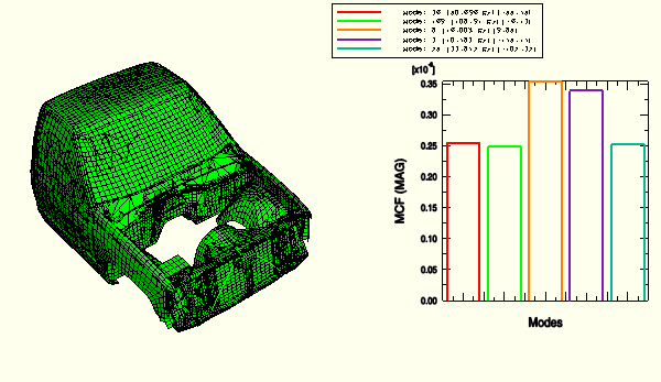
The Options tabbed page is shown in Figure 55–4:

Figure 55–4 The Options tabbed page.

The plug-in creates each type of plot in a separate viewport and names the viewport accordingly. As a result, you can select ViewportTile Vertically from the main menu bar to view all the plots at the same time. The following figures were created by the plug-in using the output database generated by a modified version of “Coupled acoustic-structural analysis of a pick-up truck,” Section 8.1.6 of the ABAQUS Example Problems Manual. The variable selected was POR, and the bar graph, polar graph, and vector graph and the ranks were generated for a frequency of 35 Hz. The analysis examined the first five ranked modes (out of 180):

Figure 55–5 shows the model that was analyzed. The bar graph indicates that Mode 36 is the significant mode at this frequency.

Figure 55–5 Bar graph of MCF for the coupled acoustic-structural analysis of a pick-up truck.

Figure 55–6 shows the X–Y plot and the projection plot. The X–Y plot shows the magnitude of the modal contribution factor at all frequencies. The projection plot shows the projection of the modal contribution factor on the total response at all frequencies. For example, mode 169 becomes more significant at 110 Hz.

Figure 55–6 X–Y and projection plots of MCF for the coupled acoustic-structural analysis of a pick-up truck.

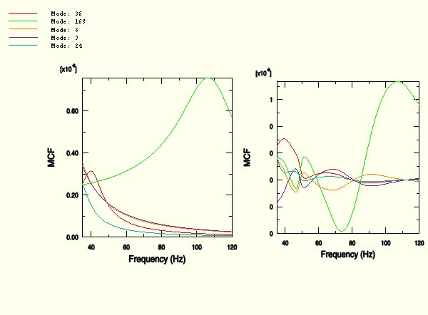
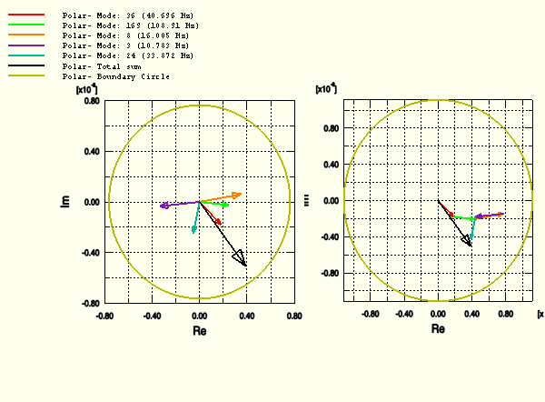
Figure 55–7 shows the polar graph and the vector graph. The bar graph shows that the magnitude of mode 36 is less than the magnitude of mode 8; however, the polar plot shows that mode 36 is more in phase with the total response (the vector sum of all the modal contributions). As a result, mode 36 contributes more to the total magnitude than mode 8 at 35 Hz and consequently ranks higher.

Figure 55–7 Polar and vector graphs of MCF for the coupled acoustic-structural analysis of a pick-up truck.