Products: ABAQUS/Standard ABAQUS/CAE
Warning: Error indicator output variables are approximate and do not represent an accurate or conservative estimate of your solution error. The quality of an error indicator can be particularly poor if your mesh is coarse. The error indicator quality improves as you refine the mesh; however, you should never interpret these variables as indicating what the value of a solution variable would be upon further refinement of the mesh.
Error indicator output variables:
are whole element variables;
indicate error in a solution quantity (the base solution) and have units of the base solution;
are typically requested through adaptive remeshing rules, where they provide necessary feedback to ABAQUS/CAE to adaptively remesh your model;
can be requested separately from ABAQUS/CAE adaptive remeshing and used to obtain indications of discretization errors in your model;
can be normalized by forms of the base solution to obtain nondimensional, such as percentage, indicators of error;
can increase your analysis solution time significantly;
are computed through the patch recovery technique of Zienkiewicz and Zhu, (1987); and
are available in ABAQUS/Standard but not ABAQUS/Explicit.
For all but trivial analyses the finite element discretization of a model domain will provide an approximation to the exact solution. To aid you in understanding the extent and spatial distribution of the error in your finite element solution, ABAQUS/Standard provides a set of error indicator output variables. ABAQUS computes the error indicators and writes them to the output database as whole element variables.
Error indicator variables are the basis of the adaptive remeshing process. They provide information to ABAQUS/CAE that describes where to refine a mesh to approach or achieve desired error indicator targets. In addition, ABAQUS/CAE uses the error indicator variables to determine where the mesh can be coarsened without introducing unacceptable errors.
ABAQUS error indicator variables provide a measure of the local error resulting from your mesh discretization. A number of error indicators are available. Each error indicator, ![]() , provides an indication of error in a particular base solution variable,
, provides an indication of error in a particular base solution variable, ![]() . Table 12.3.2–1 shows the available error indicator variables and the corresponding base solution variables.
. Table 12.3.2–1 shows the available error indicator variables and the corresponding base solution variables.
Table 12.3.2–1 Error indicator variables and their corresponding base solution variables.
| Solution Quantity | Error indicator variable ( | Base solution variable ( |
|---|---|---|
| Element energy density | ENDENERI | ENDEN |
| Mises stress | MISESERI | MISESAVG |
| Equivalent plastic strain | PEEQERI | PEEQAVG |
| Plastic strain | PEERI | PEAVG |
| Creep strain | CEERI | CEAVG |
| Heat flux | HFLERI | HFLAVG |
| Electric flux | EFLERI | EFLAVG |
| Electric potential gradient | EPGERI | EPGAVG |
For example, the Mises stress error indicator, MISESERI, provides an indicator of error in the Mises stress variable MISESAVG. ABAQUS uses the base solution variable to normalize the error indicator. When you create a remeshing rule and request a particular error indicator, ABAQUS automatically writes the corresponding base solution variable to the output database.
| Input File Usage: | Use either of the following options to request error indicator variable output outside of use with adaptive remeshing: |
*OUTPUT, FIELD *ELEMENT OUTPUT |
| ABAQUS/CAE Usage: | Use the following option to specify error indicator variables in your adaptive remeshing specification: |
Mesh module: Create Remeshing Rule: Step and Indicator or use the following option to request error indicator variable output outside of use with adaptive remeshing: Step module: Output |
You will typically choose which error indicator variables are used to control adaptive remeshing based on the type of analysis and the nature of the loading.
Certain variables apply naturally to certain types of analyses. For example, the heat flux indicator (HFLERI) is used in analyses with temperature degrees of freedom. When selecting error indicator variables in the Remeshing Rule editor in ABAQUS/CAE (see “What are remeshing rules?,” Section 17.11.1 of the ABAQUS/CAE User's Manual), your choices will be restricted to variables available for the selected procedure type.
Some error indicator variables only indicate discretization error at the current analysis time—the particular increment in a step. Other error indicator variables provide a record of the solution history up to the current analysis time. For example, if your simulation involves non-proportional loading or a significantly nonlinear response, you will typically see better adaptive remeshing results when using error indicator variables that record the solution history. Table 12.3.2–2 lists the error indicator variables and indicates whether they record the solution history.
Table 12.3.2–2 The error indicator variables that record the solution history.
| Solution Quantity | Error indicator variable ( | Records the solution history? |
|---|---|---|
| Element energy density | ENDENERI | Yes |
| Mises stress | MISESERI | No |
| Equivalent plastic strain | PEEQERI | Yes |
| Plastic strain | PEERI | No |
| Creep strain | CEERI | No |
| Heat flux | HFLERI | No |
| Electric flux | EFLERI | No |
| Electric potential gradient | EPGERI | No |
By default, when you create a remeshing rule, error indicators are specified for the final increment of the final step of your analysis and adaptive remeshing is based on error indicators in this final increment. When you select an error indicator that records the solution history, this default error indicator specification is appropriate for almost all analyses. However, for other error indicator variables that do not record the solution history, you may find it appropriate (for multi-step cases with non-proportional loading, for example) to define mutiple remeshing rules for the same region, with each rule applied to a different step.
The examples that follow provide simple illustrations of typical cases and show appropriate choices of error indicator output variables.
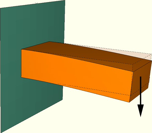
Figure 12.3.2–1 illustrates the simplest load case, where the load is proportional to the step time and the model's response is linear. In this case the solution at the final increment would be proportional to any other increment. Therefore, it is appropriate to base the remeshing on the value of the error indicator in the last increment for any choice of error indicator variable.
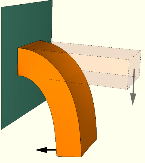
Figure 12.3.2–2 illustrates a more general case, where the model has a nonlinear response—in this case resulting from a geometric nonlinearity—and the loading is monotonic but not generally proportional to the step time.
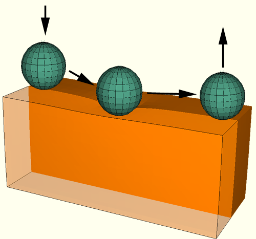
The response of the model is slightly more general because the solution at a particular increment is not proportional to the solution at the final increment. However, the value of the error indicator output in the final increment still reflects the extreme of the model's response to the load history. Therefore, it is appropriate to base the remeshing on the value of the error indicator in the last increment for any choice of error indicator variable.Figure 12.3.2–3 illustrates a case where the loading characteristics change dramatically during the analysis.
Your choice of error indicator in this case will depend on the material model. The element energy density error indicator, ENDENERI, will account for the complexity of load history (and lead to an adapted mesh that provides an accurate solution through the analysis) regardless of the material type. If plastic deformation occurs, you also have the option to use the equivalent plastic strain, PEEQERI, or plastic strain, PEERI, error indicators. Plastic strain and the plastic strain error indicator generally do not capture history effects; for example, they do not account for peak straining in models undergoing symmetric strain reversals. This example, however, involves no strain reversals; therefore, PEERI would be a valid error indicator choice.
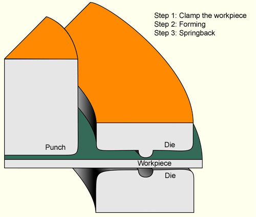
Figure 12.3.2–4 illustrates a further generalization of a general response. Here, a forming operation is simulated, and different steps are used for different stages of the operation.
In this case the response of the model varies from step to step. You will typically want the error indicator to capture the extreme of the model's response to the load history adequately. However, you do not know if any particular increment captures this extreme. Therefore, you should select an error indicator variable that records the solution history.
The patch recovery techniques that ABAQUS uses to calculate the error indicator variables can have a significant impact on the analysis solution time, of the order of 10–20% of an equation solver iteration. In particular, the element energy density is calculated after each increment and is more costly than the other error indicator variables. Therefore, you should select only those variables needed for your analysis, and you should select the element energy density error indicator only when you need to account for history dependencies (see “Choosing the error indicator variables”).
When interpreting error indicator output, you should remember that the adequacy and accuracy of your analysis depend on many factors, including mesh discretization errors, time integration errors, modeling assumptions, etc. You should perform a detailed study of your analysis methods and assumptions as part of any error assessment. This study could include, but should not be limited to, a mesh refinement study. Error indicators and the adaptive remeshing functionality of ABAQUS/CAE can help you automate your mesh refinement study.
The error indicator variable itself has the same units as the base solution variable; for example, the Mises error indicator, MISESERI, is expressed in units of stress. Your error indicator results, therefore, provide a measure you can compare directly to measures of design interest, such as stress.
You can use corresponding error indicator and base solution variables, ![]() and
and ![]() , respectively, to compute a field of local, normalized error indicators:
, respectively, to compute a field of local, normalized error indicators:
![]()
![]()
Normalized forms of an error indicator are not available directly through the error indicator output variables; however, you can calculate normalized measures using the Visualization module of ABAQUS/CAE (ABAQUS/Viewer) to operate on field output data. For more information, see “Building valid field output expressions,” Section 24.6.1 of the ABAQUS/CAE User's Manual. Alternatively, you can use the ABAQUS Scripting Interface to read the error indicator and the base solution from the output database and calculate normalized forms. For more information, see Chapter 8, “Using the ABAQUS Scripting Interface to access an output database,” of the ABAQUS Scripting User's Manual.
When you are calculating the normalized form of an error indicator, you should be aware that local values of the base solution values can be small or zero. Therefore, you should also consider other appropriate normalization approaches, such as normalizing based on a global norm of the base solution variable as opposed to local element values. Your choice of a global norm (a simple average, for example) and the corresponding effective domain (a region near a stress riser, for example) depends on your particular design or analysis goal.