Products: ABAQUS/Explicit ABAQUS/CAE
An Eulerian adaptive mesh domain:
is used to model material flowing through the mesh; and
typically has two Eulerian boundary regions, one inflow and one outflow, connected by Lagrangian and/or sliding boundary regions.
The adaptive meshing technique in ABAQUS/Explicit is robust if the mesh is underconstrained: the modeling techniques presented in this section are intended to provide guidance in properly defining Eulerian models.
ALE adaptive mesh constraints should be applied normal to an Eulerian boundary region; otherwise, the motion of the mesh on the boundary is ambiguous. If no mesh constraints are applied normal to the boundary, ABAQUS/Explicit will treat the region as if it were sliding, and the mesh will follow the material normal to the boundary.
Although there are no restrictions on specifying adaptive mesh constraints at nodes on an Eulerian boundary region, the following guidelines should be followed in most cases:
Mesh constraints should be applied to every node on the Eulerian boundary region, including the corners and edges.
Mesh constraints should be applied either only normal to the Eulerian boundary region or in every direction. Mesh constraints should not be specified in only the direction tangential to an Eulerian boundary region; such constraints are ambiguous and may result in undesirable motion of the mesh at the boundary.
Loads and boundary conditions on Eulerian boundaries act on the material that instantaneously coincides with the mesh at the surface. When used in combination with spatial adaptive mesh constraints, physically meaningful Eulerian flow conditions can be defined.
The material flowing into an adaptive mesh domain through an Eulerian boundary will have the same stress and material state as the material in the elements immediately adjacent to the boundary. Therefore, it is important to maintain the stress and material state in those elements at the desired values (which in many cases will be zero, to simulate stress-free material entering the Eulerian domain). To accomplish this goal:
position the inflow boundary far enough upstream from high solution gradients to ensure that the response at the inflow boundary is smooth, and
apply sufficient mesh and material constraints at the boundary (as described later in this section).
To be physically meaningful, the size and shape of the inflow boundary region must be maintained. For example, applying sufficient constraints is crucial for steady-state process simulations where the cross-section of the workpiece entering the adaptive mesh domain is known and affects the response downstream. The types of constraints appropriate for an inflow boundary depend on whether the precise location of the inflow boundary region is known or whether it is part of the solution.
In many problems the area, shape, and position of the inflow boundary are known a priori. For example, in the steady-state analysis of a forward extrusion process, an inflow Eulerian boundary can be used to model the flow of material into the adaptive mesh domain. The size of the inflow boundary is based on the known billet cross-section, and the location of the inflow boundary is fixed because of the confined conditions on the material.
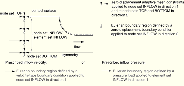
When the area, shape, and location of the inflow boundary are known, both material and mesh constraints should be applied. Figure 12.2.4–1 shows a typical model setup for a two-dimensional forward extrusion problem where either a prescribed mass flow rate or a prescribed uniform pressure is applied to a known inflow boundary. Apply boundary conditions at all nodes on the inflow boundary region to prescribe material constraints in the directions tangential to the boundary surface. Preventing motion of the material tangential to the inflow boundary helps to maintain the stress and material state of the elements adjacent to the Eulerian boundary.
Apply adaptive mesh constraints in the normal direction at all nodes on the inflow boundary. In addition, apply mesh constraints in all tangential directions at the edges and corners surrounding the Eulerian boundary region. These constraints fix the location and size of the cross-sectional area at the inflow boundary.
If a nonuniform boundary condition or load is applied to the material at the inflow boundary or if the initial material state in the elements adjacent to the boundary is nonuniform in the tangential direction, apply tangential mesh constraints to the nodes strictly in the interior of the Eulerian boundary region.
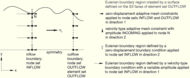
Although the application of mesh and material constraints tangential to and along the edges and corners of an inflow Eulerian boundary may appear to be redundant, they are actually independent. For example, consider a long billet with a variable cross-section, as shown in Figure 12.2.4–2.
The adaptive mesh domain, with its inflow and outflow Eulerian boundary regions, is assumed to represent a portion of the billet along its length. The entire billet moves with a rigid body velocity along its length (x-direction) so that material flows into one Eulerian boundary and out the other. Boundary conditions are applied to the material at the inflow boundary to maintain this velocity. Mesh constraints are applied normal to the inflow and outflow boundary regions. The mesh constraint applied in the y-direction at node N is used to prescribe the known variable incoming cross-section of the material. The motion of this node does not affect the velocity field of the material entering the domain.Sometimes, the location of the inflow boundary region is known only approximately; its precise location will be determined from the solution. For these problems, apply adaptive mesh constraints only in the direction normal to the Eulerian boundary region. In the absence of tangential mesh constraints at the edges and corners of the Eulerian boundary region, ABAQUS/Explicit will move these edges and corners with the material in the tangential direction but with the mesh constraints in the normal direction. Therefore, material constraints should be applied using multi-point constraints (see “General multi-point constraints,” Section 28.2.2) or linear constraint equations (see “Linear constraint equations,” Section 28.2.1) to preserve the cross-sectional area of the inflow boundary.
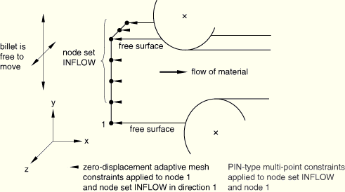
For example, consider a steady-state rolling simulation with multiple rollers in an asymmetric configuration, as shown in Figure 12.2.4–3.
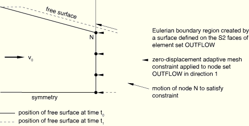
It may be impractical to extend the analysis domain as far as the guides on the upstream side, but spatially fixing the inflow boundary at an arbitrary position in the y- and z-directions may cause unrealistic stress on the workpiece as it finds an equilibrium position between the rollers. Mesh constraints are applied normal to the Eulerian boundary region to fix the position of the inflow boundary relative to the rollers in the x-direction. Material constraints (applied with a PIN MPC) are used to ensure that material enters the domain at a uniform velocity and that the cross-section does not rotate. The material constraints will maintain the cross-sectional shape of the section while allowing it to move laterally to the correct equilibrium position. Since tangential mesh constraints are not used, the mesh will follow the material in the directions tangential to the Eulerian boundary region.Typically, adaptive mesh constraints should be applied only in the direction normal to the surface on an Eulerian boundary region that acts as an outflow boundary. No tangential mesh constraints should be applied to the edges or corners of an outflow boundary adjacent to a Lagrangian (or sliding) boundary region acting as a free surface. In contrast to inflow boundaries, the cross-section of an outflow boundary adjacent to a free surface is determined by the solution in the domain. At the edge or corner where an Eulerian boundary region meets a Lagrangian or sliding boundary region, ABAQUS/Explicit will satisfy the applied mesh constraint normal to the Eulerian boundary region and the inherent mesh constraint normal to the Lagrangian or sliding boundary region simultaneously, thus correctly handling the evolution of the free surface adjacent to the outflow boundary. Figure 12.2.4–4 shows the evolution of an outflow boundary from ![]() to
to ![]() , where material continues to flow through the outflow boundary.
, where material continues to flow through the outflow boundary.
No special material boundary conditions are required at outflow Eulerian boundaries. Boundary conditions tangential to the outflow boundary are recommended only if they are the same as those defined upstream (e.g., a symmetry plane running along the length of an Eulerian domain). However, to improve convergence to the steady-state solution in steady-state process simulations, it is often useful to constrain the material velocity to be uniform normal to the outflow boundary using multi-point constraints or linear constraint equations.
Although it is rarely appropriate, an Eulerian boundary region can act as both an inflow and an outflow boundary at different times during the same analysis step. Adaptive mesh constraints and material boundary conditions at such a boundary should be chosen to be physically meaningful for both inflow and outflow situations.
For each node on the edges and corners of an Eulerian boundary region that does not have mesh constraints tangential to the boundary surface, ABAQUS/Explicit will determine in each adaptive mesh increment whether the boundary at the node is acting as an inflow or an outflow boundary. If an inflow condition is detected, the node will move with the material in the tangential direction but with the mesh constraints in the normal direction. If an outflow condition is detected, the movement of the node will both follow the adjacent Lagrangian boundary region and satisfy the mesh constraint normal to the Eulerian boundary region.
Many applications using Eulerian adaptive mesh domains, including the simulation of steady-state processes, have a primary direction of material flow and use a control volume approach to model the process zone. These problems usually include two Eulerian boundary regions, representing an inflow boundary and outflow boundary. The remaining surfaces between the Eulerian boundaries can be either Lagrangian or sliding boundary regions. Determining which type of boundary region to use between the two Eulerian boundary regions depends on the type of load or boundary condition that is required:
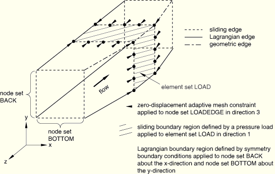
Use a sliding boundary region to define boundary conditions or loads that act at a spatial location on a portion of the surface along the length of the control volume. Apply adaptive mesh constraints to fix the mesh spatially in the flow direction (and possibly in the direction transverse to the flow). For example, a distributed pressure can be applied around the circumference of the control volume, as shown in Figure 12.2.4–5.
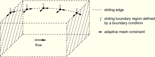
The distributed pressure load is defined using a sliding boundary region. Mesh constraints are applied to fix the boundary region spatially in the flow direction. Similarly, a concentrated load could be applied to a specific spatial location to model the effect of a very sharp body pressing into the workpiece at a known location with a known force.Use a sliding boundary region to define boundary conditions or loads that act along the entire length of the Eulerian control volume between the inflow and outflow boundaries and act in a spatial manner transversely to the flow. If the load acts on only a portion of the surface in the transverse direction, it may be necessary to apply mesh constraints in the direction transverse to the flow. For example, a boundary condition that acts as a knife edge along the length of the domain is shown in Figure 12.2.4–6. Mesh constraints are applied in the transverse direction (and, if the line of application is curved, along the line) to keep the boundary condition fixed spatially.
Use a Lagrangian boundary region (default) to define boundary conditions or loads that act along the entire length of the surface of the Eulerian control volume between the inflow and outflow boundary and act in a Lagrangian manner transversely to the flow. In three dimensions, symmetry conditions should typically act in a Lagrangian manner transverse to the flow direction. In many cases geometric edges will prevent material from flowing off the symmetry plane and onto the free surface. However, since geometric edges can be deactivated as surfaces flatten, Lagrangian boundary regions should be used to define the symmetry planes for these types of problems. In Figure 12.2.4–5 quarter-symmetry is assumed, and the symmetry planes are defined using Lagrangian boundary regions. The resulting Lagrangian edges that run from one Eulerian boundary to the other separate the symmetry planes from the free surface.
Boundary conditions or loads that act on only a specific portion of the material between the inflow and outflow boundaries cannot usually be modeled for problems utilizing Eulerian control volumes. Since the mesh underneath the load or boundary condition must follow the material, it will eventually be restricted by the Eulerian boundary. This treatment of loads and boundary conditions is not usually consistent with a steady-state model and should not arise in practical simulations using Eulerian adaptive mesh domains.