Product: ABAQUS/Standard

User subroutine MPC:
is called to impose a user-defined multi-point constraint and is intended for use when general constraints cannot be defined with one of the MPC types provided by ABAQUS/Standard;
can use only degrees of freedom that also exist on an element somewhere in the same model (methods for overcoming this limitation are discussed below);
can generate linear as well as nonlinear constraints;
allows definition of constraints involving finite rotations; and
makes it possible to switch constraints on and off during an analysis.
There are two methods for coding this routine. By default, the subroutine operates in a degree of freedom mode. In this mode each call to this subroutine allows one individual degree of freedom to be constrained. Alternatively, you can specify that the subroutine operate in a nodal mode. In this mode each call to this subroutine allows a set of constraints to be imposed all at once; that is, on multiple degrees of freedom of the dependent node. In either case, the routine will be called for each user-subroutine-defined multi-point constraint or set of constraints. See “General multi-point constraints,” Section 28.2.2 of the ABAQUS Analysis User's Manual, for details.
In geometrically nonlinear analyses ABAQUS/Standard compounds three-dimensional rotations based on a finite-rotation formulation and not by simple addition of the individual rotation components (see “Conventions,” Section 1.2.2 of the ABAQUS Analysis User's Manual, and “Rotation variables,” Section 1.3.1 of the ABAQUS Theory Manual). An incremental rotation involving one component usually results in changes in all three total rotation components. Therefore, any general constraint that involves large three-dimensional rotations should be implemented using the nodal mode of user subroutine MPC. The single degree of freedom version of user subroutine MPC can be used for geometrically linear problems, geometrically nonlinear problems with planar rotations, and constraints that do not involve rotation components.
The degrees of freedom involved in user MPCs must appear on some element or ABAQUS/Standard MPC type in the model: user MPCs cannot use degrees of freedom that have not been introduced somewhere on an element. For example, a mesh that uses only continuum (solid) elements cannot have user MPCs that involve rotational degrees of freedom. The simplest way to overcome this limitation is to introduce an element somewhere in the model that uses the required degrees of freedom but does not affect the solution in any other way. Alternatively, if the degrees of freedom are rotations, they can be activated by the use of a library BEAM-type MPC somewhere in the model.
When a local coordinate system (“Transformed coordinate systems,” Section 2.1.5 of the ABAQUS Analysis User's Manual) and a user MPC are both used at a node, the variables at the node are first transformed before the MPC is imposed. Therefore, user-supplied MPCs must be based on the transformed degrees of freedom. The local-to-global transformation matrices ![]() for the individual nodes:
for the individual nodes:
![]()
This version of user subroutine MPC allows for one individual degree of freedom to be constrained and, thus, eliminated at a time. The constraint can be quite general and nonlinear of the form:
![]()
You must provide, at all times, two items of information in user subroutine MPC:
A list of degree of freedom identifiers at the nodes that are listed in the corresponding multi-point constraint definition. This list corresponds to ![]() , etc. in the constraint as given above.
, etc. in the constraint as given above.
An array of the derivatives
![]()
In addition, you can provide the value of the dependent degree of freedom ![]() as a function of the independent degrees of freedom
as a function of the independent degrees of freedom ![]() etc. If this value is not provided, ABAQUS/Standard will update
etc. If this value is not provided, ABAQUS/Standard will update ![]() based on the linearized form of the constraint equation as
based on the linearized form of the constraint equation as
      SUBROUTINE MPC(UE,A,JDOF,MDOF,N,JTYPE,X,U,UINIT,MAXDOF,
     * LMPC,KSTEP,KINC,TIME,NT,NF,TEMP,FIELD,LTRAN,TRAN)
C
      INCLUDE 'ABA_PARAM.INC'
C
      DIMENSION A(N),JDOF(N),X(6,N),U(MAXDOF,N),UINIT(MAXDOF,N),
     * TIME(2),TEMP(NT,N),FIELD(NF,NT,N),LTRAN(N),TRAN(3,3,N)


      user coding to define UE, A, JDOF, and, optionally, LMPC


      RETURN
      END
SUBROUTINE MPC(UE,A,JDOF,MDOF,N,JTYPE,X,U,UINIT,MAXDOF,
* LMPC,KSTEP,KINC,TIME,NT,NF,TEMP,FIELD,LTRAN,TRAN)
C
INCLUDE 'ABA_PARAM.INC'
C
DIMENSION A(N),JDOF(N),X(6,N),U(MAXDOF,N),UINIT(MAXDOF,N),
* TIME(2),TEMP(NT,N),FIELD(NF,NT,N),LTRAN(N),TRAN(3,3,N)
user coding to define UE, A, JDOF, and, optionally, LMPC
RETURN
ENDA(N)
An array containing the derivatives of the constraint function,
![]()
JDOF(N)
An array containing the degree of freedom identifiers at the nodes that are involved in the constraint. For example, if ![]() is the z-displacement at a node, give JDOF(1) = 3; if
is the z-displacement at a node, give JDOF(1) = 3; if ![]() is the x-displacement at a node, give JDOF(2) = 1. The coding in the subroutine must define N entries in JDOF, where N is defined below.
is the x-displacement at a node, give JDOF(2) = 1. The coding in the subroutine must define N entries in JDOF, where N is defined below.
UE
This variable is passed in as the total value of the eliminated degree of freedom, ![]() . This variable will either be zero or have the current value of
. This variable will either be zero or have the current value of ![]() based on the linearized constraint equation, depending at which stage of the iteration the user subroutine is called. If the constraint is linear and is used in a small-displacement analysis (nonlinear geometric effects are not considered) or in a perturbation analysis, this variable need not be defined: ABAQUS/Standard will compute
based on the linearized constraint equation, depending at which stage of the iteration the user subroutine is called. If the constraint is linear and is used in a small-displacement analysis (nonlinear geometric effects are not considered) or in a perturbation analysis, this variable need not be defined: ABAQUS/Standard will compute ![]() as
as
LMPC
Set this variable to zero to avoid the application of the multi-point constraint. The MPC will be applied if the variable is not changed. This variable must be set to zero every time the subroutine is called if the user MPC is to remain deactivated. This MPC variable is useful for switching the MPC on and off during an analysis. However, the option should be used with care: switching off an MPC may cause a sudden disturbance in equilibrium, which can lead to convergence problems. If this variable is used to switch on an MPC during an analysis, the variable UE should be defined; otherwise, the constraint may not be satisfied properly.
MDOF
Maximum number of active degrees of freedom per node involved in the MPC. For the degree of freedom mode of user subroutine MPC, MDOF= 1.
N
Number of degrees of freedom that are involved in the constraint, defined as the number of nodes given in the corresponding multi-point constraint definition. If more than one degree of freedom at a node is involved in a constraint, the node must be repeated as needed or, alternatively, the nodal mode should be used.
JTYPE
Constraint identifier given for the corresponding multi-point constraint definition.
X(6,N)
An array containing the original coordinates of the nodes involved in the constraint.
U(MAXDOF,N)
An array containing the values of the degrees of freedom at the nodes involved in the constraint. These values will be either the values at the end of the previous iteration or the current values based on the linearized constraint equation, depending at which stage of the iteration the user subroutine is called.
UINIT(MAXDOF,N)
An array containing the values at the beginning of the current iteration of the degrees of freedom at the nodes involved in the constraint. This information is useful for decision-making purposes when you do not want the outcome of a decision to change during the course of an iteration. For example, there are constraints in which the degree of freedom to be eliminated changes during the course of the analysis, but it is necessary to prevent the choice of the dependent degree of freedom from changing during the course of an iteration.
MAXDOF
Maximum degree of freedom number at any node in the analysis. For example, for a coupled temperature-displacement analysis with continuum elements, MAXDOF will be equal to 11.
KSTEP
Step number.
KINC
Increment number within the step.
TIME(1)
Current value of step time.
TIME(2)
Current value of total time.
NT
Number of positions through a section where temperature or field variable values are stored at a node. In a mesh containing only continuum elements, NT=1. For a mesh containing shell or beam elements, NT is the largest of the values specified for the number of temperature points in the shell or beam section definition (or 2 for temperatures specified together with gradients for shells or two-dimensional beams, 3 for temperatures specified together with gradients for three-dimensional beams).
NF
Number of different predefined field variables requested for any node (including field variables defined as initial conditions).
TEMP(NT,N)
An array containing the temperatures at the nodes involved in the constraint. This array is not used for a heat transfer, coupled temperature-displacement, or coupled thermal-electrical analysis since the temperatures are degrees of freedom of the problem.
FIELD(NF,NT,N)
An array containing all field variables at the nodes involved in the constraint.
LTRAN(N)
An integer array indicating whether the nodes in the MPC are transformed. If LTRAN(I)=1, a transformation is applied to node I; if LTRAN(I)=0, no transformation is applied.
TRAN(3,3,N)
An array containing the local-to-global transformation matrices for the nodes used in the MPC. If no transformation is present at node I, TRAN(*,*,I) is the identity matrix.
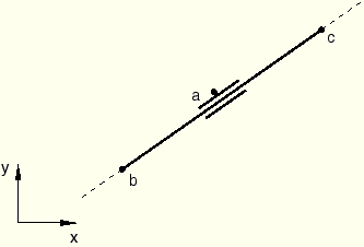
An example of a nonlinear single degree of freedom MPC is a geometrically nonlinear two-dimensional slider involving nodes a, b, and c. The constraint forces node a to be on the straight line connecting nodes b and c (see Figure 1–1).
The constraint equation can be written in the form![]()
![]()
![]()
To prevent the choice of either ![]() or
or ![]() as the dependent degree of freedom from changing during the course of an iteration, the orientation of the segment
as the dependent degree of freedom from changing during the course of an iteration, the orientation of the segment ![]() is tested based on the geometry at the beginning of the iteration. The dependent degree of freedom is allowed to change from increment to increment.
is tested based on the geometry at the beginning of the iteration. The dependent degree of freedom is allowed to change from increment to increment.
Suppose the above multi-point constraint is defined as type 1, with nodes a, a, b, b, c, c. The user subroutine MPC could be coded as follows:
      SUBROUTINE MPC(UE,A,JDOF,MDOF,N,JTYPE,X,U,UINIT,MAXDOF,
     * LMPC,KSTEP,KINC,TIME,NT,NF,TEMP,FIELD,LTRAN,TRAN)
C
      INCLUDE 'ABA_PARAM.INC'
C
      DIMENSION A(N),JDOF(N),X(6,N),U(MAXDOF,N),UINIT(MAXDOF,N),
     * TIME(2),TEMP(NT,N),FIELD(NF,NT,N),LTRAN(N),TRAN(3,3,N)
      PARAMETER( PRECIS = 1.D-15 )
C
      IF (JTYPE .EQ. 1) THEN
        DYBC0 = X(2,5) + UINIT(2,5) - X(2,3) - UINIT(2,3)
        DXBC0 = X(1,3) + UINIT(1,3) - X(1,5) - UINIT(1,5)
        DYBC = X(2,5) + U(2,5) - X(2,3) - U(2,3)
        DXBC = X(1,3) + U(1,3) - X(1,5) - U(1,5)
        A(3) = X(2,1) + U(2,1) - X(2,5) - U(2,5)
        A(4) = X(1,5) + U(1,5) - X(1,1) - U(1,1)
        A(5) = X(2,3) + U(2,3) - X(2,1) - U(2,1)
        A(6) = X(1,1) + U(1,1) - X(1,3) - U(1,3)
        JDOF(3) = 1
        JDOF(4) = 2
        JDOF(5) = 1
        JDOF(6) = 2
        IF (ABS(DYBC0).LE.PRECIS .AND. ABS(DXBC0).LE.PRECIS) THEN
C
C         POINTS B AND C HAVE COLLAPSED. DO NOT APPLY CONSTRAINT.
C
          LMPC = 0
        ELSE IF (ABS(DXBC0) .LT. ABS(DYBC0)) THEN
C
C         MAKE U_A DEPENDENT DOF.
C
          JDOF(1) = 1
          JDOF(2) = 2
          A(1) = DYBC
          A(2) = DXBC
          UE = A(5)A(2)/A(1) + X(1,3) + U(1,3) - X(1,1)
        ELSE
C
C         MAKE V_A DEPENDENT DOF.
C
          JDOF(1) = 2
          JDOF(2) = 1
          A(1) = DXBC
          A(2) = DYBC
          UE = -A(6)A(2)/A(1) + X(2,3) + U(2,3) - X(2,1)
        END IF
      END IF
C
      RETURN
      END
The nodal version of user subroutine MPC allows for multiple degrees of freedom of a node to be eliminated simultaneously. The set of constraints can be quite general and nonlinear, of the form
![]()
NDEP is the number of dependent degrees of freedom that are involved in the constraint and should have a value between 1 and MDOF, which is the number of active degrees of freedom per node in the analysis. N is the number of nodes involved in the constraint. The scalar constraint functions ![]() can also be considered as a vector function
can also be considered as a vector function ![]() , and the first set of degrees of freedom
, and the first set of degrees of freedom ![]() in the vector function
in the vector function ![]() will be eliminated to impose the constraint. The sets
will be eliminated to impose the constraint. The sets ![]() ,
, ![]() , etc. are the independent degrees of freedom at nodes 2, 3, etc. involved in the constraint. The set
, etc. are the independent degrees of freedom at nodes 2, 3, etc. involved in the constraint. The set ![]() must be composed of NDEP degrees of freedom at the first node of the MPC definition. For example, if the dependent degrees of freedom are the x-displacement, the z-displacement, and the y-rotation at the first node,
must be composed of NDEP degrees of freedom at the first node of the MPC definition. For example, if the dependent degrees of freedom are the x-displacement, the z-displacement, and the y-rotation at the first node, ![]() .
. ![]() ,
, ![]() etc. can be composed of any number of degrees of freedom, depending on which ones play a role in the constraint, and need not be of the same size; for example,
etc. can be composed of any number of degrees of freedom, depending on which ones play a role in the constraint, and need not be of the same size; for example, ![]() and
and ![]() .
.
The dependent node can also reappear as an independent node in the MPC. However, since the dependent degrees of freedom of this node will be eliminated, they cannot be used as independent degrees of freedom in this MPC. For example, if the rotations at node a are constrained by the MPC, the displacements of node a can still be used as independent degrees of freedom in the MPC, but the rotations themselves cannot. Similarly, the degrees of freedom that will be eliminated to impose the constraint cannot be used in subsequent kinematic constraints (multi-point constraints, linear equation constraints, or boundary conditions). The MPCs are imposed in the order given in the input for this purpose.
The nodal version of user subroutine MPC was designed with the application of nonlinear constraints involving large three-dimensional rotations in mind. Due to the incremental nature of the solution procedure in ABAQUS/Standard, a linearized set of constraints
![]()
![]()
You must provide, at all times, two items of information in subroutine MPC:
A matrix of degree of freedom identifiers at the nodes that are listed in the corresponding multi-point constraint definition. The columns of this matrix correspond to ![]() , etc. in the set of constraints as given above, where unused entries are padded with zeros. The number of nonzero entries in
, etc. in the set of constraints as given above, where unused entries are padded with zeros. The number of nonzero entries in ![]() will implicitly determine the number of dependent degrees of freedom, NDEP.
will implicitly determine the number of dependent degrees of freedom, NDEP.
The matrices representing the linearized constraint function with respect to the degrees of freedom involved. These matrices are needed for the redistribution of loads from degrees of freedom ![]() to the other degrees of freedom and for the elimination of
to the other degrees of freedom and for the elimination of ![]() from the system matrices. For constraints that do not involve three-dimensional rotations and constraints with planar rotations, these matrices can be readily obtained from the derivatives of the total constraint function with respect to the degrees of freedom involved:
from the system matrices. For constraints that do not involve three-dimensional rotations and constraints with planar rotations, these matrices can be readily obtained from the derivatives of the total constraint function with respect to the degrees of freedom involved:
![]()
![]()
      SUBROUTINE MPC(UE,A,JDOF,MDOF,N,JTYPE,X,U,UINIT,MAXDOF,
     * LMPC,KSTEP,KINC,TIME,NT,NF,TEMP,FIELD,LTRAN,TRAN)
C
      INCLUDE 'ABA_PARAM.INC'
C
      DIMENSION UE(MDOF),A(MDOF,MDOF,N),JDOF(MDOF,N),X(6,N),
     * U(MAXDOF,N),UINIT(MAXDOF,N),TIME(2),TEMP(NT,N),
     * FIELD(NF,NT,N),LTRAN(N),TRAN(3,3,N)


      user coding to define JDOF, UE, A and, optionally, LMPC


      RETURN
      END
SUBROUTINE MPC(UE,A,JDOF,MDOF,N,JTYPE,X,U,UINIT,MAXDOF,
* LMPC,KSTEP,KINC,TIME,NT,NF,TEMP,FIELD,LTRAN,TRAN)
C
INCLUDE 'ABA_PARAM.INC'
C
DIMENSION UE(MDOF),A(MDOF,MDOF,N),JDOF(MDOF,N),X(6,N),
* U(MAXDOF,N),UINIT(MAXDOF,N),TIME(2),TEMP(NT,N),
* FIELD(NF,NT,N),LTRAN(N),TRAN(3,3,N)
user coding to define JDOF, UE, A and, optionally, LMPC
RETURN
ENDJDOF(MDOF,N)
Matrix of degrees of freedom identifiers at the nodes involved in the constraint. Before each call to MPC, ABAQUS/Standard will initialize all of the entries of JDOF to zero. All active degrees of freedom for a given column (first index ranging from 1 to MDOF) must be defined starting at the top of the column with no zeros in between. A zero will mark the end of the list for that column. The number of nonzero entries in the first column will implicitly determine the number of dependent degrees of freedom (NDEP). For example, if the dependent degrees of freedom are the z-displacement, the x-rotation, and the z-rotation at the first node, NDEP![]() and
and
![]()
![]()
A(MDOF,MDOF,N)
Submatrices of coefficients of the linearized constraint function,
![]()
UE(NDEP)
This array is passed in as the total value of the eliminated degrees of freedom, ![]() . This array will either be zero or contain the current values of
. This array will either be zero or contain the current values of ![]() based on the linearized constraint equations, depending at which stage of the iteration the user subroutine is called. For small-displacement analysis or perturbation analysis this array need not be defined: ABAQUS/Standard will compute
based on the linearized constraint equations, depending at which stage of the iteration the user subroutine is called. For small-displacement analysis or perturbation analysis this array need not be defined: ABAQUS/Standard will compute ![]() as
as
LMPC
Set this variable to zero to avoid the application of the multi-point constraint. If the variable is not changed, the MPC will be applied. This variable must be set to zero every time the subroutine is called if the user MPC is to remain deactivated. This MPC variable is useful for switching the MPC on and off during an analysis. This option should be used with care: switching off an MPC may cause a sudden disturbance in equilibrium, which can lead to convergence problems.
MDOF
Number of active degrees of freedom per node in the analysis. For example, for a coupled temperature-displacement analysis with two-dimensional continuum elements, the active degrees of freedom are 1, 2, and 11 and, hence, MDOF will be equal to 3.
N
Number of nodes involved in the constraint. The value of N is defined as the number of nodes given in the corresponding multi-point constraint definition.
JTYPE
Constraint identifier given for the corresponding multi-point constraint definition.
X(6,N)
An array containing the original coordinates of the nodes involved in the constraint.
U(MAXDOF,N)
An array containing the values of the degrees of freedom at the nodes involved in the constraint. These values will either be the values at the end of the previous iteration or the current values based on the linearized constraint equation, depending at which stage of the iteration the user subroutine is called.
UINIT(MAXDOF,N)
An array containing the values at the beginning of the current iteration of the degrees of freedom at the nodes involved in the constraint. This information is useful for decision-making purposes when you do not want the outcome of a decision to change during the course of an iteration. For example, there are constraints in which the degrees of freedom to be eliminated change during the course of the analysis, but it is necessary to prevent the choice of the dependent degrees of freedom from changing during the course of an iteration.
MAXDOF
Maximum degree of freedom number at any node in the analysis. For example, for a coupled temperature-displacement analysis with continuum elements, MAXDOF is equal to 11.
KSTEP
Step number.
KINC
Increment number within the step.
TIME(1)
Current value of step time.
TIME(2)
Current value of total time.
NT
Number of positions through a section where temperature or field variable values are stored at a node. In a mesh containing only continuum elements, NT=1. For a mesh containing shell or beam elements, NT is the largest of the values specified for the number of temperature points in the shell or beam section definition (or 2 for temperatures specified together with gradients for shells or two-dimensional beams, 3 for temperatures specified together with gradients for three-dimensional beams).
NF
Number of different predefined field variables requested for any node (including field variables defined as initial conditions).
TEMP(NT,N)
An array containing the temperatures at the nodes involved in the constraint. This array is not used for a heat transfer, coupled temperature-displacement, or coupled thermal-electrical analysis since the temperatures are degrees of freedom of the problem.
FIELD(NF,NT,N)
An array containing all field variables at the nodes involved in the constraint.
LTRAN(N)
An integer array indicating whether the nodes in the MPC are transformed. If LTRAN(I)=1, a transformation is applied to node I; if LTRAN(I)=0, no transformation is applied.
TRAN(3,3,N)
An array containing the local-to-global transformation matrices for the nodes used in the MPC. If no transformation is present at node I, TRAN(*,*,I) is the identity matrix.
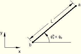
As an example of a nonlinear MPC, consider the insertion of a rigid beam in a large-displacement, planar (two-dimensional) problem. This MPC is the two-dimensional version of library BEAM-type MPC. It can be implemented as a set of three different single degree of freedom MPCs or as a single nodal MPC. Here, the second method will be worked out because it is simpler and requires less data input.
Let a and b (see Figure 1–2) be the ends of the beam, with a the dependent end.
The rigid beam will then define both components of displacement and the rotation at a in terms of the displacements and rotation at end b according to the set of equations:
In terms of the original positions ![]() and
and ![]() of a and b,
of a and b,
![]()
![]()

If the above multi-point constraint is defined as type 1 with nodes a and b, the user subroutine MPC could be coded as follows:
      SUBROUTINE MPC(UE,A,JDOF,MDOF,N,JTYPE,X,U,UINIT,MAXDOF,LMPC,
     * KSTEP,KINC,TIME,NT,NF,TEMP,FIELD,LTRAN,TRAN)
C
      INCLUDE 'ABA_PARAM.INC'
C
      DIMENSION UE(MDOF),A(MDOF,MDOF,N),JDOF(MDOF,N),X(6,N),
     * U(MAXDOF,N),UINIT(MAXDOF,N),TIME(2),TEMP(NT,N),
     * FIELD(NF,NT,N),LTRAN(N),TRAN(3,3,N)
C
      IF (JTYPE .EQ. 1) THEN
        COSFIB = COS(U(6,2))
        SINFIB = SIN(U(6,2))
        ALX = X(1,1) - X(1,2)
        ALY = X(2,1) - X(2,2)
C
        UE(1) = U(1,2) + ALX*(COSFIB-1.) - ALY*SINFIB
        UE(2) = U(2,2) + ALY*(COSFIB-1.) + ALX*SINFIB
        UE(3) = U(6,2)
C
        A(1,1,1) =  1.
        A(2,2,1) =  1.
        A(3,3,1) =  1.
        A(1,1,2) = -1.
        A(1,3,2) =  ALX*SINFIB + ALY*COSFIB
        A(2,2,2) = -1.
        A(2,3,2) = -ALX*COSFIB + ALY*SINFIB
        A(3,3,2) = -1.
C
        JDOF(1,1) = 1
        JDOF(2,1) = 2
        JDOF(3,1) = 6
        JDOF(1,2) = 1
        JDOF(2,2) = 2
        JDOF(3,2) = 6
      END IF
C
      RETURN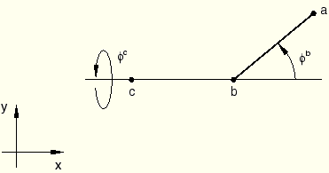
ENDAs an example of a nonlinear MPC involving finite rotations, consider a two-dimensional constant velocity joint that might be part of a robotics application. Let a, b, c (see Figure 1–3) be the nodes making up the joint, with a the dependent node.
The joint is operated by prescribing an axial rotation![]()
In geometrically linear problems compound rotations are obtained simply as the linear superposition of individual rotation vectors. Consider the geometry depicted in Figure 1–3 and assume that the infinitesimal rotations ![]() and
and ![]() are applied at c and b, respectively. The rotation
are applied at c and b, respectively. The rotation ![]() at a will simply be the sum of the vector
at a will simply be the sum of the vector ![]() to the vector
to the vector ![]() rotated by an angle
rotated by an angle ![]() about the z-axis. Thus, the linearized constraint can be written directly as
about the z-axis. Thus, the linearized constraint can be written directly as

Since degrees of freedom 4 (![]() ), 5(
), 5(![]() ), and 6(
), and 6(![]() ) appear in this constraint, there must be an element in the mesh that uses these degrees of freedom—a B31 beam element, for example. The MPC subroutine has been coded with just this information. In this case ABAQUS/Standard updates the dependent rotation field,
) appear in this constraint, there must be an element in the mesh that uses these degrees of freedom—a B31 beam element, for example. The MPC subroutine has been coded with just this information. In this case ABAQUS/Standard updates the dependent rotation field, ![]() , based on the linearized constraint equations. Although the constraint is not satisfied exactly, good results are obtained as long as the rotation increments are kept small enough. A more rigorous derivation of the linearized constraint and the exact nonlinear recovery of the dependent degrees of freedom is presented in “Rotation variables,” Section 1.3.1 of the ABAQUS Theory Manual.
, based on the linearized constraint equations. Although the constraint is not satisfied exactly, good results are obtained as long as the rotation increments are kept small enough. A more rigorous derivation of the linearized constraint and the exact nonlinear recovery of the dependent degrees of freedom is presented in “Rotation variables,” Section 1.3.1 of the ABAQUS Theory Manual.
If the above multi-point constraint is defined as type 1 with nodes a, b, and c, user subroutine MPC could be coded as follows:
      SUBROUTINE MPC(UE,A,JDOF,MDOF,N,JTYPE,X,U,UINIT,MAXDOF,LMPC,
     * KSTEP,KINC,TIME,NT,NF,TEMP,FIELD,LTRAN,TRAN)
C
      INCLUDE 'ABA_PARAM.INC'
C
      DIMENSION UE(MDOF),A(MDOF,MDOF,N),JDOF(MDOF,N),X(6,N),
     * U(MAXDOF,N),UINIT(MAXDOF,N),TIME(2),TEMP(NT,N),
     * FIELD(NF,NT,N),LTRAN(N),TRAN(3,3,N)
C
      IF (JTYPE .EQ. 1) THEN
        A(1,1,1) =  1.
        A(2,2,1) =  1.
        A(3,3,1) =  1.
        A(3,1,2) = -1.
        A(1,1,3) = -COS(U(6,2))
        A(2,1,3) = -SIN(U(6,2))
C
        JDOF(1,1) = 4
        JDOF(2,1) = 5
        JDOF(3,1) = 6
        JDOF(1,2) = 6
        JDOF(1,3) = 4
      END IF
C
      RETURN
      END