This section contains a conceptual and an algorithmic description of the ABAQUS/Explicit analysis product as well as a discussion on the advantages of the method.
This section attempts to provide some conceptual understanding of how forces propagate through a model when using the explicit dynamics method. In this illustrative example we consider the propagation of a stress wave along a rod modeled with three elements, as shown in Figure 3–1. We study the state of the rod as we increment through time.
In the first time increment node 1 has an acceleration, ![]() , as a result of the concentrated force,
, as a result of the concentrated force, ![]() , applied to it. The acceleration causes node 1 to have a velocity,
, applied to it. The acceleration causes node 1 to have a velocity, ![]() , which, in turn, causes a strain rate,
, which, in turn, causes a strain rate, ![]() , in element 1. The increment of strain,
, in element 1. The increment of strain, ![]() , in element 1 is obtained by integrating the strain rate through the time of increment 1. The total strain,
, in element 1 is obtained by integrating the strain rate through the time of increment 1. The total strain, ![]() , is the sum of the initial strain,
, is the sum of the initial strain, ![]() , and the increment in strain. In this case the initial strain is zero. Once the element strain has been calculated, the element stress,
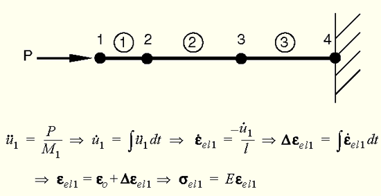
, and the increment in strain. In this case the initial strain is zero. Once the element strain has been calculated, the element stress, ![]() , is obtained by applying the material constitutive model. For a linear elastic material the stress is simply the elastic modulus times the total strain. This process is shown in Figure 3–2. Nodes 2 and 3 do not move in the first increment since no force is applied to them.
, is obtained by applying the material constitutive model. For a linear elastic material the stress is simply the elastic modulus times the total strain. This process is shown in Figure 3–2. Nodes 2 and 3 do not move in the first increment since no force is applied to them.
Figure 3–2 Configuration at the end of increment 1 of a rod with a concentrated load, ![]() , at the free end.
, at the free end.
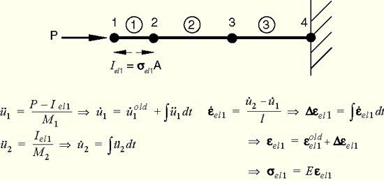
In the second increment the stresses in element 1 apply internal, element forces to the nodes associated with element 1, as shown in Figure 3–3. These element stresses are then used to calculate dynamic equilibrium at nodes 1 and 2.
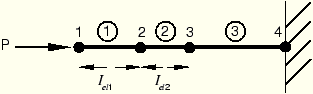
The process continues so that at the start of the third increment there are stresses in both elements 1 and 2, and there are forces at nodes 1, 2, and 3, as shown in Figure 3–4. The process continues until the analysis reaches the desired total time.
ABAQUS/Explicit uses a central difference rule to integrate the equations of motion explicitly through time, using the kinematic conditions at one increment to calculate the kinematic conditions at the next increment. At the beginning of the increment the program solves for dynamic equilibrium, which states that the nodal mass matrix, ![]() , times the nodal accelerations,
, times the nodal accelerations, ![]() , equals the total nodal forces (the difference between the external applied forces,
, equals the total nodal forces (the difference between the external applied forces, ![]() , and internal element forces,
, and internal element forces, ![]() ):
):
![]()
The accelerations at the beginning of the current increment (time ![]() ) are calculated as
) are calculated as
![]()
Since the explicit procedure always uses a diagonal, or lumped, mass matrix, solving for the accelerations is trivial; there are no simultaneous equations to solve. The acceleration of any node is determined completely by its mass and the net force acting on it, making the nodal calculations very inexpensive.
The accelerations are integrated through time using the central difference rule, which calculates the change in velocity assuming that the acceleration is constant. This change in velocity is added to the velocity from the middle of the previous increment to determine the velocities at the middle of the current increment:
![]()
The velocities are integrated through time and added to the displacements at the beginning of the increment to determine the displacements at the end of the increment:
![]()
Thus, satisfying dynamic equilibrium at the beginning of the increment provides the accelerations. Knowing the accelerations, the velocities and displacements are advanced “explicitly” through time. The term “explicit” refers to the fact that the state at the end of the increment is based solely on the displacements, velocities, and accelerations at the beginning of the increment. This method integrates constant accelerations exactly. For the method to produce accurate results, the time increments must be quite small so that the accelerations are nearly constant during an increment. Since the time increments must be small, analyses typically require many thousands of increments. Fortunately, each increment is inexpensive because there are no simultaneous equations to solve. Most of the computational expense lies in the element calculations to determine the internal forces of the elements acting on the nodes. The element calculations include determining element strains and applying material constitutive relationships (the element stiffness) to determine element stresses and, consequently, internal forces.
Here is a summary of the explicit dynamics algorithm:
Nodal calculations.
Dynamic equilibrium.
![]()
Integrate explicitly through time.
![]()
![]()
Element calculations.
Compute element strain increments, ![]() , from the strain rate,
, from the strain rate, ![]() .
.
Compute stresses, ![]() , from constitutive equations.
, from constitutive equations.
![]()
Assemble nodal internal forces, ![]() .
.
Set ![]() to
to ![]() and return to Step 1.
and return to Step 1.
The explicit method is especially well-suited to solving high-speed dynamic events that require many small increments to obtain a high-resolution solution. If the duration of the event is short, the solution can be obtained efficiently.
Contact conditions and other extremely discontinuous events are readily formulated in the explicit method and can be enforced on a node-by-node basis without iteration. The nodal accelerations can be adjusted to balance the external and internal forces during contact.
The most striking feature of the explicit method is the lack of a global tangent stiffness matrix, which is required with implicit methods. Since the state of the model is advanced explicitly, iterations and tolerances are not required.