Two types of shell elements are available in ABAQUS: conventional shell elements and continuum shell elements. Conventional shell elements discretize a reference surface by defining the element's planar dimensions, its surface normal, and its initial curvature. The nodes of a conventional shell element, however, do not define the shell thickness; the thickness is defined through section properties. Continuum shell elements, on the other hand, resemble three-dimensional solid elements in that they discretize an entire three-dimensional body yet are formulated so that their kinematic and constitutive behavior is similar to conventional shell elements. Continuum shell elements are more accurate in contact modeling than conventional shell elements, since they employ two-sided contact taking into account changes in thickness. For thin shell applications, however, conventional shell elements provide superior performance.
In this manual only conventional shell elements are discussed. Henceforth, we will refer to them simply as “shell elements.” For more information on continuum shell elements, see “Shell elements: overview,” Section 23.6.1 of the ABAQUS Analysis User's Manual.
The shell thickness is required to describe the shell cross-section and must be specified. In addition to specifying the shell thickness, you can choose to have the stiffness of the cross-section calculated during the analysis or once at the beginning of the analysis.
If you choose to have the stiffness calculated during the analysis, ABAQUS uses numerical integration to calculate the stresses and strains independently at each section point (integration point) through the thickness of the shell, thus allowing nonlinear material behavior. For example, an elastic-plastic shell may yield at the outer section points while remaining elastic at the inner section points. The location of the single integration point in an S4R (4-node, reduced integration) element and the configuration of the section points through the shell thickness are shown in Figure 5–1.
You can specify any odd number of section points through the shell thickness when the properties are integrated during the analysis. By default, ABAQUS uses five section points through the thickness of a homogeneous shell, which is sufficient for most nonlinear design problems. However, you should use more section points in some complicated simulations, especially when you anticipate reversed plastic bending (nine is normally sufficient in this case). For linear problems three section points provide exact integration through the thickness. However, calculating the material stiffness once at the beginning of the analysis is more efficient for linear elastic shells.
The material behavior must be linear elastic when the stiffness of the cross-section is calculated only at the beginning of the simulation. In this case all calculations are done in terms of the resultant forces and moments across the entire cross-section. If you request stress or strain output, ABAQUS provides default output for the bottom surface, the midplane, and the top surface.
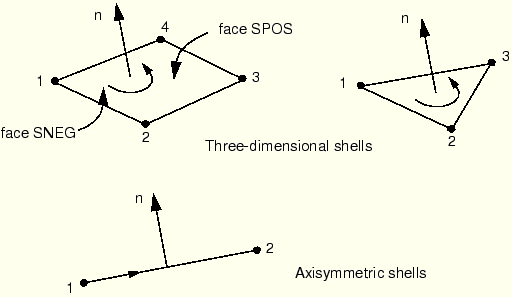
The connectivity of the shell element defines the direction of the positive normal, as shown in Figure 5–2.
For axisymmetric shell elements the positive normal direction is defined by a 90° counterclockwise rotation from the direction going from node 1 to node 2. For three-dimensional shell elements the positive normal is given by the right-hand rule going around the nodes in the order in which they appear in the element definition.
The “top” surface of a shell is the surface in the positive normal direction and is called the SPOS face for contact definition. The “bottom” surface is in the negative direction along the normal and is called the SNEG face for contact definition. Normals should be consistent among adjoining shell elements.
The positive normal direction defines the convention for element-based pressure load application and output of quantities that vary through the shell thickness. A positive element-based pressure load applied to a shell element produces a load that acts in the direction of the positive normal. (The element-based pressure load convention for shell elements is opposite to that for continuum elements; the surface-based pressure load conventions for shell and continuum elements are identical. For more on the difference between element-based and surface-based distributed loads, see “Distributed loads,” Section 27.4.3 of the ABAQUS Analysis User's Manual.)
Shells in ABAQUS (with the exception of element types S3/S3R, S3RS, S4R, S4RS, S4RSW, and STRI3) are formulated as true curved shell elements; true curved shell elements require special attention to accurate calculation of the initial surface curvature. ABAQUS automatically calculates the surface normals at the nodes of every shell element to estimate the initial curvature of the shell. The surface normal at each node is determined using a fairly elaborate algorithm, which is discussed in detail in “Defining the initial geometry of conventional shell elements,” Section 23.6.3 of the ABAQUS Analysis User's Manual.
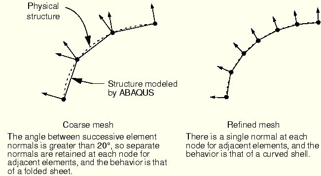
With a coarse mesh as shown in Figure 5–3, ABAQUS may determine several independent surface normals at the same node for adjoining elements. Physically, multiple normals at a single node mean that there is a fold line between the elements sharing the node. While it is possible that you intend to model such a structure, it is more likely that you intend to model a smoothly curved shell; ABAQUS will try to smooth the shell by creating an averaged normal at a node.
The basic smoothing algorithm used is as follows: if the normals at a node for each shell element attached to the node are within 20° of each other, the normals will be averaged. The averaged normal will be used at that node for all elements attached to the node. If ABAQUS cannot smooth the shell, a warning message is issued in the data (.dat) file.
There are two methods that can be used to override the default algorithm. To introduce fold lines into a curved shell or to model a curved shell with a coarse mesh, either give the components of ![]() as the 4th, 5th, and 6th data values following the nodal coordinates (this method requires manually editing the input file created by ABAQUS/CAE in a text editor); or specify the normal direction directly with the *NORMAL option (this option can be added using the ABAQUS/CAE Keywords Editor; see “Cross-section orientation,” Section 6.1.2). If both methods are used, the latter takes precedence. See “Defining the initial geometry of conventional shell elements,” Section 23.6.3 of the ABAQUS Analysis User's Manual, for further details.
as the 4th, 5th, and 6th data values following the nodal coordinates (this method requires manually editing the input file created by ABAQUS/CAE in a text editor); or specify the normal direction directly with the *NORMAL option (this option can be added using the ABAQUS/CAE Keywords Editor; see “Cross-section orientation,” Section 6.1.2). If both methods are used, the latter takes precedence. See “Defining the initial geometry of conventional shell elements,” Section 23.6.3 of the ABAQUS Analysis User's Manual, for further details.
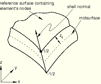
The reference surface of the shell is defined by the shell element's nodes and normal definitions. When modeling with shell elements, the reference surface is typically coincident with the shell's midsurface. However, many situations arise in which it is more convenient to define the reference surface as offset from the shell's midsurface. For example, surfaces created in CAD packages usually represent either the top or bottom surface of the shell body. In this case it may be easier to define the reference surface to be coincident with the CAD surface and, therefore, offset from the shell's midsurface.
Shell offsets can also be used to define a more precise surface geometry for contact problems where shell thickness is important. Another situation where the offset from the midsurface may be important is when a shell with continuously varying thickness is modeled. In this case defining the nodes at the shell midplane can be difficult. If one surface is smooth while the other is rough, as in some aircraft structures, it is easiest to use shell offsets to define the nodes at the smooth surface.
Offsets can be introduced by specifying an offset value that is defined as a fraction of the shell thickness measured from the shell's midsurface to the shell's reference surface, as shown in Figure 5–4.
The degrees of freedom for the shell are associated with the reference surface. All kinematic quantities, including the element's area, are calculated there. Large offset values for curved shells may lead to a surface integration error, affecting the stiffness, mass, and rotary inertia for the shell section. For stability purposes ABAQUS/Explicit also automatically augments the rotary inertia used for shell elements on the order of the offset squared, which may result in errors in the dynamics for large offsets. When large offsets from the shell's midsurface are necessary, use multi-point constraints or rigid body constraints instead.